Writing
Machine Learning (3) — Least Squares
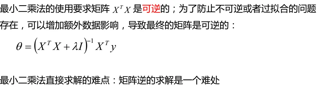
Least squares concept, Gaussian error assumptions, household power example, and R²/MSE metrics.
Preface: Introduction to least squares and its applications.
Concept
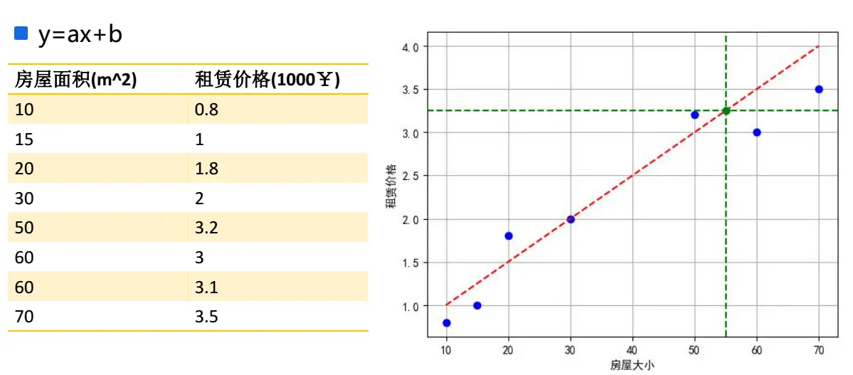
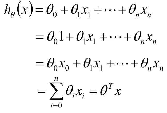
A linear model predicts via linear combinations:
Formulas:

Errors are i.i.d. Gaussian with mean 0 and variance σ².
Reason: central limit theorem—many random phenomena are sums of independent factors and tend toward normal.
Loss function:

Solution:
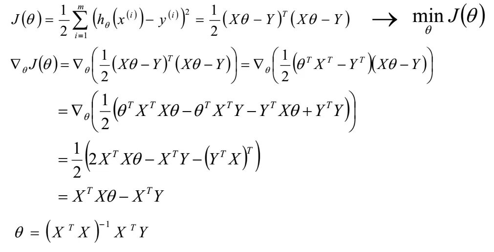
Same as the linear algebra solution.
Least Squares
Projection matrix solves inconsistent systems—same solution as above.
Example: predict household power from current. Data: http://archive.ics.uci.edu/ml/datasets/Individual+household+electric+power+consumption
from sklearn.model_selection import train_test_split
import numpy as np
import pandas as pd
from pandas import DataFrame
import matplotlib as mpl
import matplotlib.pyplot as plt
import time
#防止中文乱码
mpl.rcParams['font.sans-serif']=[u'simHei']
mpl.rcParams['axes.unicode_minus']=False
#加载数据
path = "household_power_consumption_1000.txt"
df = pd.read_csv(path,sep=";",low_memory=False)

#功率和电流之间的关系
X = df.iloc[:,2:4]
Y = df.iloc[:,5]
#数据集划分两个参数test_size表示怎么划分,random_state固定随机种子类似于在执行random模块时候,给一个随机种子random.seed(0),之后每次运行的随机数不会改变
x_train,x_test,y_train,y_test=train_test_split(X,Y,test_size=0.2,random_state=0)
#转化为矩阵形式,进行最小二乘法运算,即矩阵的运算
x1 = np.mat(x_train)
y1 = np.mat(y_train).reshape(-1,1)#转化为一列-1表示一后面1列为标准
#带入最小二乘公式求θ
theat = (x1.T*x1).I*x1.T*y1
print(theat)
#对测试集进行训练
y_hat = np.mat(x_test)*theat
#画图看看,预测值和实际值比较200个预测值之间的比较
t = np.arange(len(x_test))
plt.figure()
plt.plot(t,y_test,"r-",label=u'真实值')
plt.plot(t,y_hat,"g-",label=u'预测值')
# plt.legend(loc = 'lower right')
plt.title(u"线性回归预测功率与电流之间的关系", fontsize=20)
plt.grid(b=True)
plt.show()
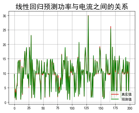
Output: θ=[[4.20324605], [1.36676171]]. Prediction plot:
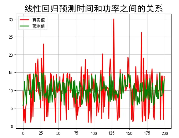
train_test_split can be implemented manually:
import random
import csv
def loadDataset(fileName,split,trainingSet=[],textSet=[]):
with open(fileName, "r") as f:
reader = csv.reader(f)
data = list(reader)
for x in range(len(data) - 1):
for y in range(4):
data[x][y] = float(data[x][y])
if random.random()
### Metrics
- R² Coefficient of determination / goodness of fit. Definition:
> The coefficient R^2 is defined as (1 - u/v), where u is the regression sum of squares ((y_true - y_pred) ** 2).sum() and v is the residual sum of squares ((y_true - y_true.mean()) ** 2).sum().
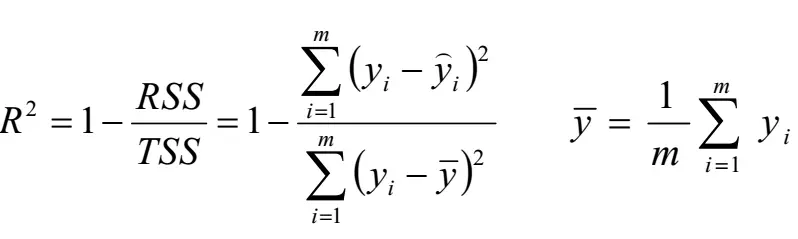
Closer to 1 → better fit. Call `lr.score(x_test, y_test)`.
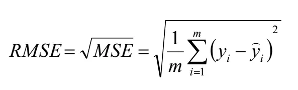
- MSE and RMSE