Deep Learning — CNN (1)

Preface: Earlier neuron connections were fully connected; with huge inputs, parameters explode and computation is heavy. CNNs mimic how humans observe—first grasp main local features—adding convolution (local perception) and pooling (feature simplification). CNNs are widely used in image classification and object recognition.

Layer Structure

• Input layer: same preprocessing as ML—common methods: 1) zero-center each dimension 2) normalize amplitudes to the same range 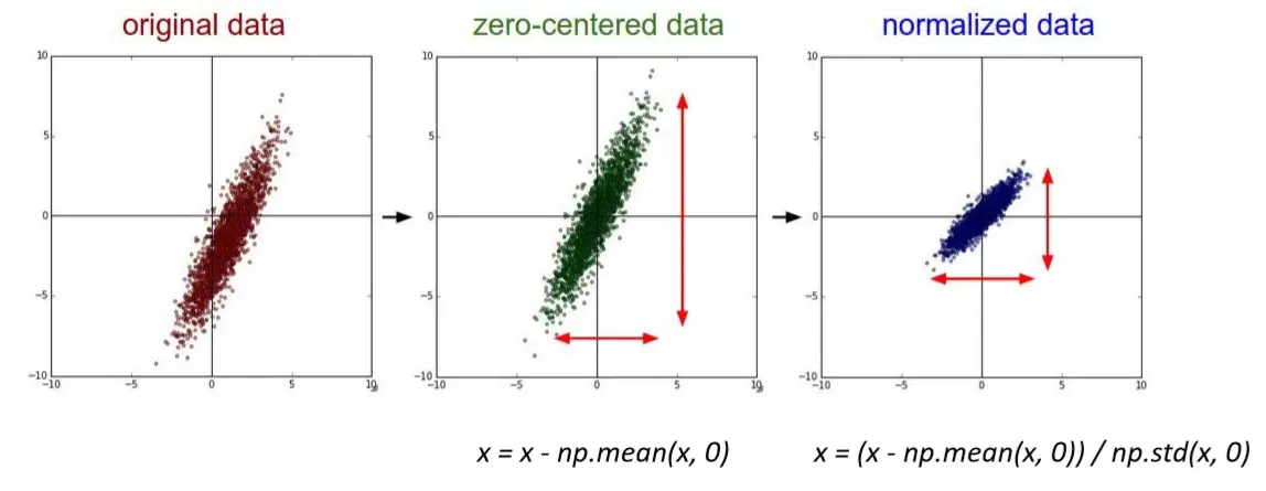3) PCA/whitening—PCA removes correlation; whitening normalizes each PCA axis 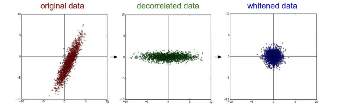Formulas: zero-mean x -= np.mean(x, axis=0); covariance cov = np.dot(x.T, x) / x.shape[0]; SVD u, s, v = np.linalg.svd(cov); PCA xrot = np.dot(x, u); x = np.dot(x, u[:, :2]); whiten x = xrot / np.sqrt(s + 1e-5). CNNs rarely use PCA/whitening; zero-mean and normalization are common. Convolution layer (CONV): ReLU. The brain processes color, shape, light, etc., in different cortical areas then merges—local observation first, global merge second. Convolution is like that local judgment. CONV principle: local connection—each neuron is a filter window sliding over local data. Concepts: depth, stride, zero-padding. Demo: http://cs231n.github.io/assets/conv-demo/index.html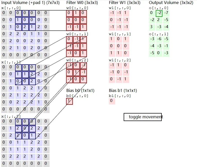 One filter views one aspect; multiple filters form depth 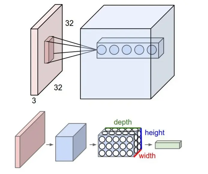CONV traits: local perception; parameter sharing (fixed weights per window); overlapping windows smooth edges; each neuron is a template; far fewer weights; convolution is inner product of window and filter then sum. Activation (ReLU): nonlinear map after convolution 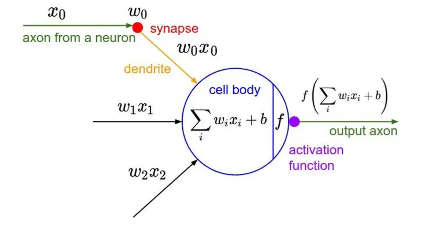Common activations:

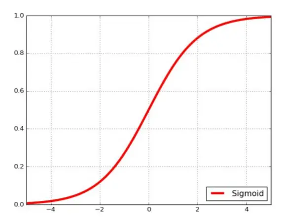
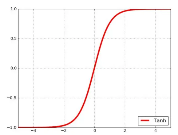
• Sigmoid: common but prone to “dead neurons” Tanh: similar issues; rarely used in CNN ReLU: zero for x≤0, y=x for x>0 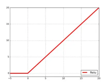Cons: unbounded—variant ReLU min(max(0,x),6); fragile—small learning rate helps. Pros: faster convergence than Sigmoid/Tanh; simple gradients; no vanishing/exploding; brain-like.

• One-sided inhibition;

• relatively wide excitation boundary;

• sparse activation;

• faster convergence;

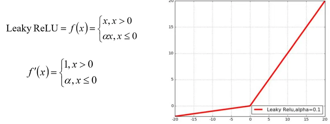
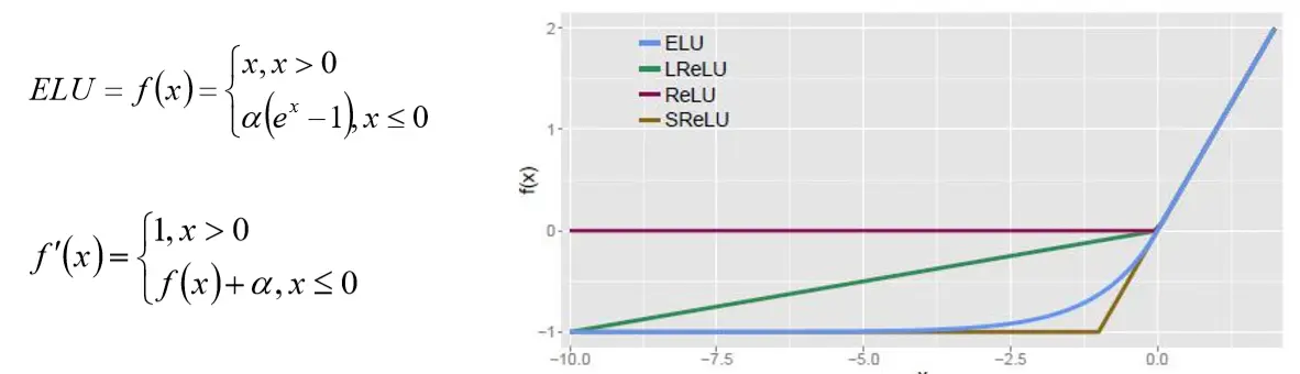
• Leaky ReLU fixes x≤0 to address dead neurons ELU Maxout: exponential fix for x≤0 vs Leaky’s linear fix Maxout (paper): extra activation layer with parameter k; pick max of k activations. Pros: simple, no saturation, fewer dead neurons. Cons: doubled parameters, heavier compute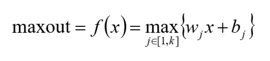

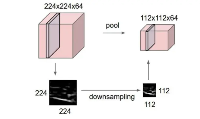
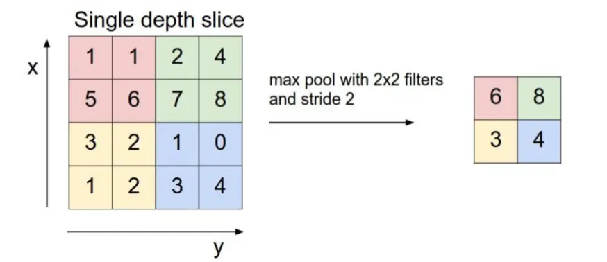
• Pooling: between conv layers; shrinks spatial size and computation; independent per feature map; Max Pooling (common) or Average Pooling

• Fully connected (FC): neurons connect to all prior activations; usually only at the tail in CNNs

CNN Traits

Pros: shared kernels, handles high dimensions; no hand-crafted features; deep nets extract rich image structure. Cons: tuning, many samples, many iterations, GPU preferred; physical meaning of layers unclear.

Parameter Initialization

Weights: small random Gaussian (mean 0, variance ~2/n); never all zeros (identical gradients). Biases: usually 0; tiny values possible with ReLU.

Overfitting Remedies

Regularization (L1/L2 on cost); Dropout—randomly drop neurons each iteration, train on subnetworks, reduce co-dependence, more robust features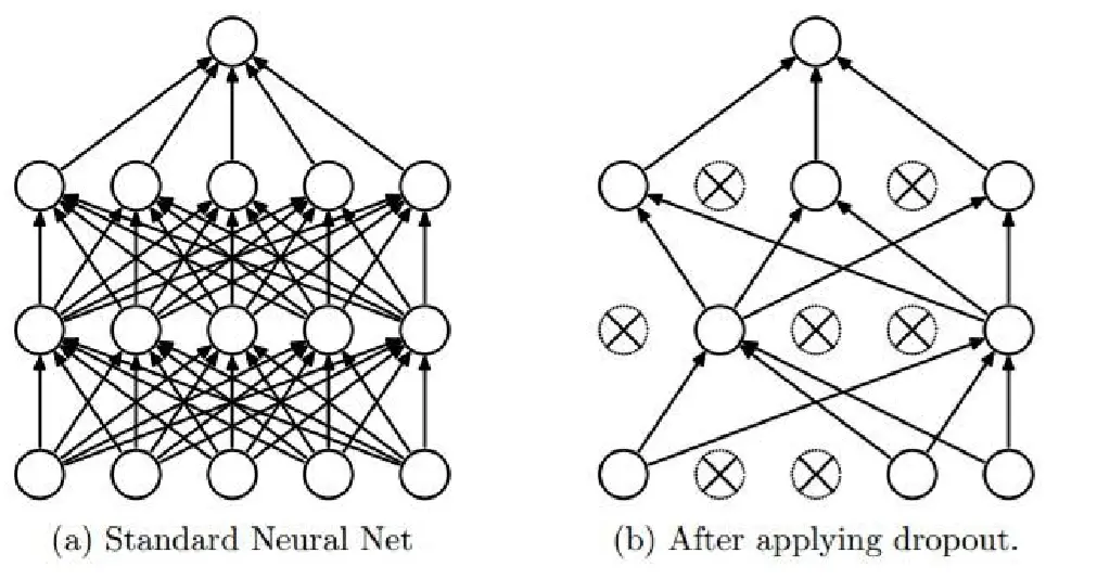

Local Response Normalization (LRN)

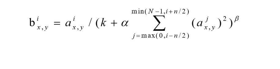
Mimics lateral inhibition; competition among local responses; larger responses stand out; after activation/pooling. For activation output at (x,y) from kernel j, sum n neighboring kernels’ activations at same position; hyperparameters k, α, β from validation (often k=2, α=10⁻⁴, β=0.75):