Mutual Information and Information Entropy

Information Entropy

Reference: Information Entropy (CSDN)

Also called Shannon entropy, introduced by Shannon in 1948. He noted that the more ordered a system, the lower its entropy; the more chaotic, the higher. Entropy measures how ordered a system is.

1. Information Content

The information carried by a single sample. The more likely an event, the less information it carries. Examples:

In the extreme case, “the sun rises in the east” is certain and carries no information.

“I ran into Jay Chou while shopping yesterday” carries a lot of information.

2. Information Entropy

The entropy formula is shown below:

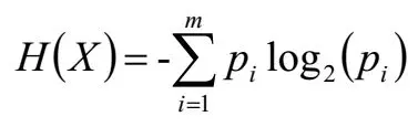
Random variable X has m events; the average number of bits needed per event is entropy. If one event has very high probability, the variable carries less information and entropy decreases.

Example: in a horse race, two groups of eight horses with win probabilities as shown:

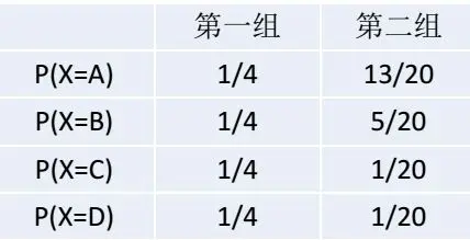
Group 1 has equal probabilities — hard to guess the winner. Group 2 clearly favors horse A. Entropy: group 1 H(X)=2, group 2 H(X)=1.336.

Conditional Entropy H(Y|X)

Overall, the expectation of entropy.

Definition: the entropy of random variable Y given condition X. Example:

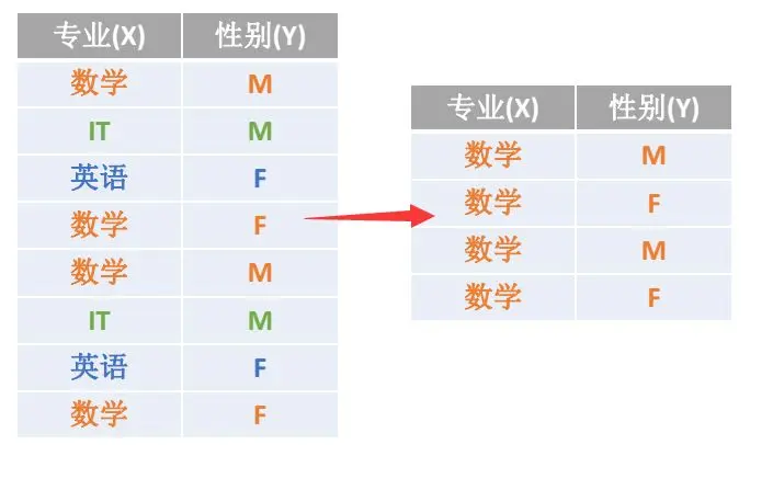
Entropy of major (when X is mathematics) H(Y|X=数学)=1. The average of H(Y|X) over all values of X is conditional entropy. Result for the example:

Mutual Information

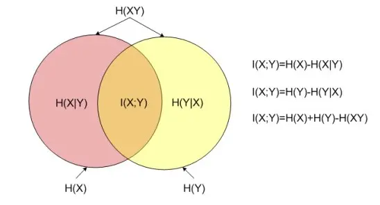
Mutual information measures: knowing X, how much uncertainty about Y is reduced (or knowing Y, how much about X).

Left and Right Neighbor Character Entropy

Compute the entropy of characters to the left (or right) of a word. We use entropy to measure how random the left-neighbor and right-neighbor sets of a text fragment are.

Example: In “吃葡萄不吐葡萄皮不吃葡萄倒吐葡萄皮” (“Eat grapes without spitting grape skins; don’t eat grapes but spit grape skins”), “葡萄” (grape) appears four times. Left neighbors: {吃, 吐, 吃, 吐}; right neighbors: {不, 皮, 倒, 皮}. By the formula, left-neighbor entropy ≈ 0.693; right-neighbor entropy ≈ 1.04. In this sentence, right neighbors are more diverse.

Viewpoint: when left entropy is low, the fragment is unlikely to be a standalone word.

On Renren user statuses, “被子” (quilt) appeared 956 times; “辈子” (lifetime) 2,330 times. Right-neighbor entropies are 3.87404 and 4.11644 — very close. But “被子” has rich left contexts: most common “晒被子” (sun the quilt) 162 times; then “的被子” 85; “条被子”, “在被子”, “床被子” 69, 64, 52; plus “叠被子”, “盖被子”, “加被子”, “新被子”, “掀被子”, “收被子”, “薄被子”, “踢被子”, “抢被子” and 100+ rarer patterns — left entropy 3.67453.

“辈子” has poor left diversity: of 2,330 occurrences, 1,276 are “一辈子” (whole life), 596 “这辈子” (this life), 235 “下辈子” (next life), 149 “上辈子” (past life), 32 “半辈子”, 10 “八辈子”, 7 “几辈子”, 6 “哪辈子”, plus 13 rarer forms. Left entropy is only 1.25963 — whether “辈子” is a word is debatable.

“下子” is more typical: of 310 uses, 294 are “一下子” (all at once), 5 “两下子”, 5 “这下子”, rest single-occurrence rare forms. Left entropy is only 0.294421 — we should not treat “下子” as a flexible word.

Some fragments have fine left neighbors but sparse right ones — e.g. “交响”, “后遗”, “鹅卵” — treating them as words is also questionable. Define a fragment’s freedom of use as the minimum of its left and right neighbor entropies.

Computation

Compute mutual information and left/right entropy with a Trie tree: The Art of Programming · 06.09

Trie Tree (Prefix Tree)

What Is a Trie?

A Trie (prefix tree or digital tree) is a tree structure. Typical uses: counting and sorting large numbers of strings (not limited to strings), often in search engines for term frequency. It minimizes redundant string comparisons and queries efficiently.

The core idea: trade space for time, using common prefixes to cut comparison cost.

Three basic properties:

• The root contains no character; every other node contains one character.
• Characters along the path from root to a node form the string for that node.
• No two children of a node share the same character.

Building the Tree

Problem: given 100,000 words of length at most 10, for each word determine whether it appeared before and, if so, at which position first. Naive approach: for each word, scan all previous words — O(n²), unacceptable at 100k scale.

Alternative thinking:

• To find “abcd”, words starting with b, c, d, f need not be considered — only those starting with a that might be “abcd”.
• Among a-prefixed words, only those with b as the second letter matter. Narrow scope repeatedly and a tree model emerges.

Given words b, abc, abd, bcd, abcd, efg, hii, we build:

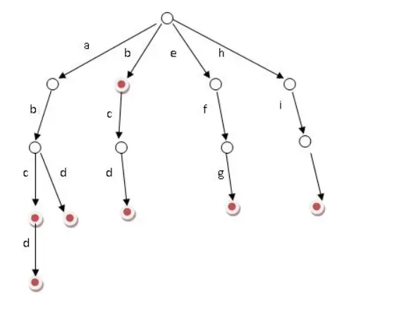
For each node, the path from root is a word. A red node means the word exists; otherwise not.

To query a word, walk from root to the node and check red. Marking red inserts the word. Query and insert share one pass, time proportional to word length (here, 10). That is a Trie.

Each level can have up to 26^i nodes. To save space, use dynamic linked lists or array-simulated dynamics. Space is at most word count × average word length.

Lookup

Tries are simple, practical structures for dictionary lookup — e.g. AJAX typeahead search boxes. A Trie stores many strings; edges are characters; branches are substrings; leaves are full strings. Unlike ordinary trees, shared prefixes share branches.

Example: inn, int, at, age, adv, ant:

• Each edge is a letter.
• Each node is a prefix; leaves are full words.
• “inn” and “int” share prefix “in” — branch root→i→in. ate, age, adv, ant share “a” — branch root→a.

Lookup is straightforward: to find “int”, follow i → in → int.

Insertion: insert each letter of each word; reuse existing prefixes or create nodes and edges. To insert “add”:

1. Prefix “a” — edge a exists; follow to node a.
2. Remaining “dd”, prefix “d” — edge d from a exists; follow to ad.
3. Final “d” — no d from ad; create child add, mark edge ad→add as d.

Problem Examples

1. A text file with about 10,000 lines, one word per line. Find the 10 most frequent words. Give the idea and time complexity.

Hint: Trie counts occurrences — O(n×le) (le = average word length). Then top 10 via a heap — O(n×lg10). Total: max(O(n×le), O(n×lg10)).

2. Hot query mining

Original: a search engine logs every query string (1–255 bytes). Assume 10 million records with high duplication — after dedup, at most 3 million unique. Higher repetition means more users and hotter queries. Find the top 10 query strings using at most 1 GB memory.

Hint: Trie with occurrence count in each node (0 if absent). Sort frequencies with a min-heap of size 10.