Machine Learning (2) — Gradient Descent

• An optimization method for unconstrained problems—recursive approximation to minimum loss. See prior notes on from directional derivatives to gradient.

• Update:

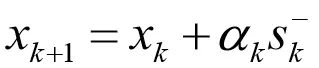
x is the variable, s is negative gradient direction, α is step size (learning rate). Cons: slow near minima; zigzag paths; weak on complex nonlinear functions.

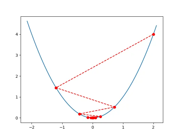
• Example: gradient descent on y=x**2:

import numpy as np
import matplotlib.pyplot as plt
import matplotlib as mpl

def f(x):
    return x**2
def h(x):
    return 2*x
X=[]
Y=[]

x=2
step=0.8
f_change=f(x)
f_current=f(x)
X.append(x)
Y.append(f_current)
while f_change>np.e**-10:
    x=x-step*h(x)
    tmp=f(x)
    f_change=np.abs(f_current-tmp)
    f_current=tmp
    X.append(x)
    Y.append(f_current)
print(X)
print(Y)
print(x,f_current)
fig = plt.figure()
a=np.arange(-2.15,2.15,0.05)
b=a**2
plt.plot(a,b)
plt.plot(X,Y,"ro--")
plt.show()

Result:

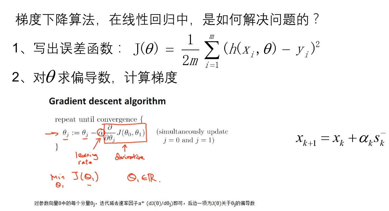
• Unknown parameters in objective:

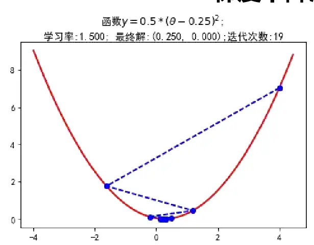
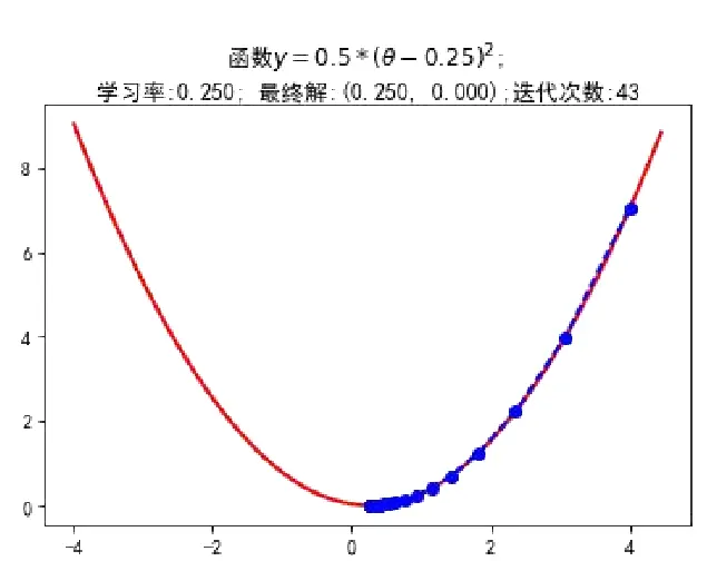
• Step size and initialization Different steps:

• Learning rate: too large may overshoot optimum; too small slows convergence.

• Initialization: different starts may reach different local minima—run multiple inits and pick lowest loss.

var ihubo = {
    nickName  : "草依山",
    site : "http://jser.me"
  }

Steps: define parameterized function, loss vs target, gradient descent for parameters minimizing loss → prediction model.