Machine Learning Explainability 01 — SHAP

Summary

This article introduces SHAP theory and gives a simple example revealing how SHAP values are computed; it then explains how to convert SHAP values into probabilities we can understand more easily.

What Is SHAP?

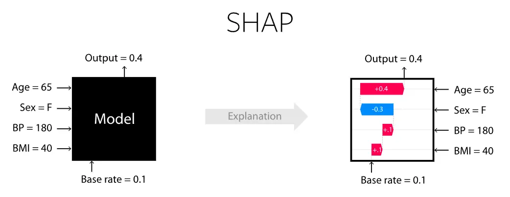
SHAP makes machine learning interpretable by computing each feature’s contribution to a prediction.

SHAP paper

GitHub link

Reference blog

What Is the Theory Behind SHAP?

Game Theory and Machine Learning

SHAP values are based on Shapley values from game theory. Game theory needs at least two things: a game and players. How does this apply to ML explainability? Given a prediction model:

• The “game” is reproducing the model’s output
• The “players” are the features in the model

Shapley quantifies each player’s contribution to the game. SHAP quantifies each feature’s contribution to the model’s prediction.

Importantly, the “game” involves a single observation. One game: one sample. SHAP is about local explainability of prediction models.

Power Set

The power set of features. Example: imagine a model (linear regression or any other algorithm) that knows a person’s age, gender, and job, and predicts income.

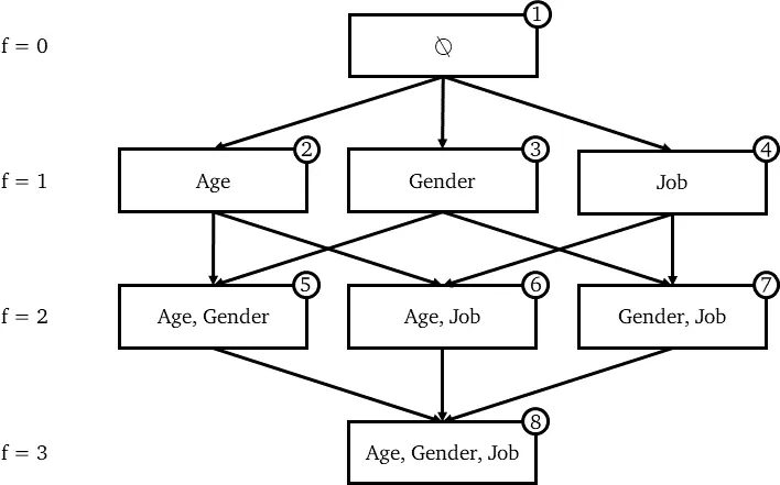
Shapley values consider outcomes for every possible coalition of players to decide one player’s importance. Here, that means every subset of features (from 0 to F, where F is the total number of features).

In mathematics this is the “power set,” representable as a directed acyclic graph.

Example

A model predicting income from age, job, and gender.

• Step 1: build the power set of features:

• Step 2: train models for each subset in the power set

• Step 3: compute the SHAP value for age on one sample. Model outputs for that sample:

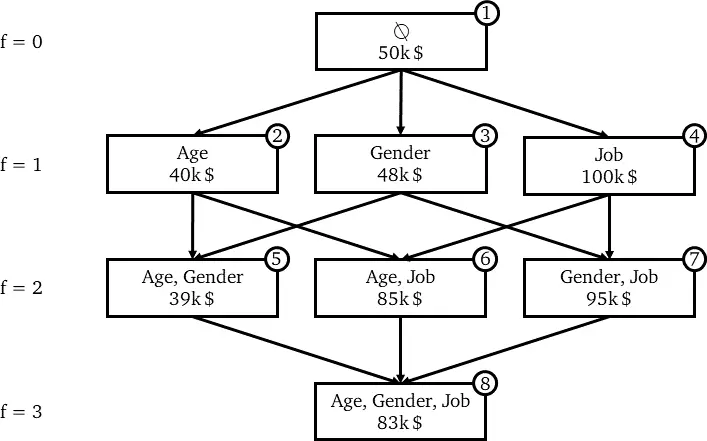
First compute age’s contribution:

Compute weights via GAG:

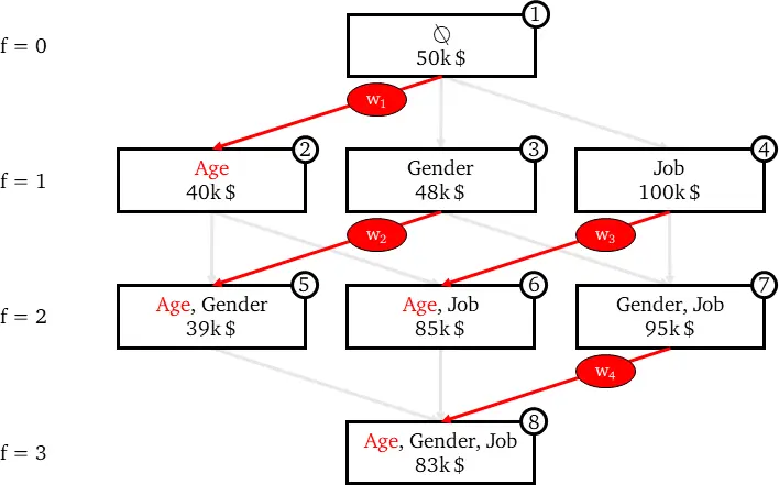
Finally obtain age’s SHAP value:

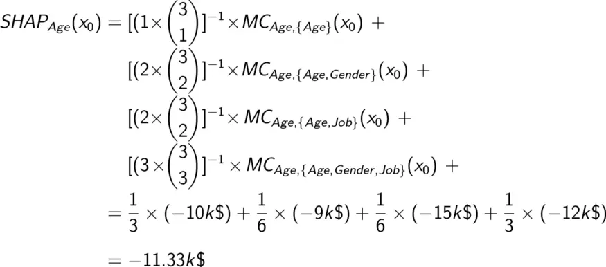
SHAP values for each feature:

SHAP_Age(x₀) = -11.33k $

SHAP_Gender(x₀) = -2.33k $

SHAP_Job(x₀) = +46.66k $

SHAP Formula

• For a single sample, SHAP values are often shown as:

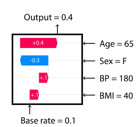
Or:

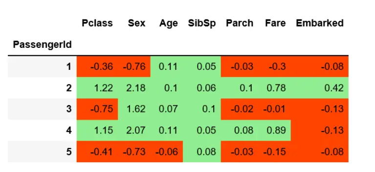
Or in table form:

Presenting SHAP Values as Probabilities

Reference blog. Example: convert SHAP values to probabilities, then take differences to see whether a feature increased survival probability.

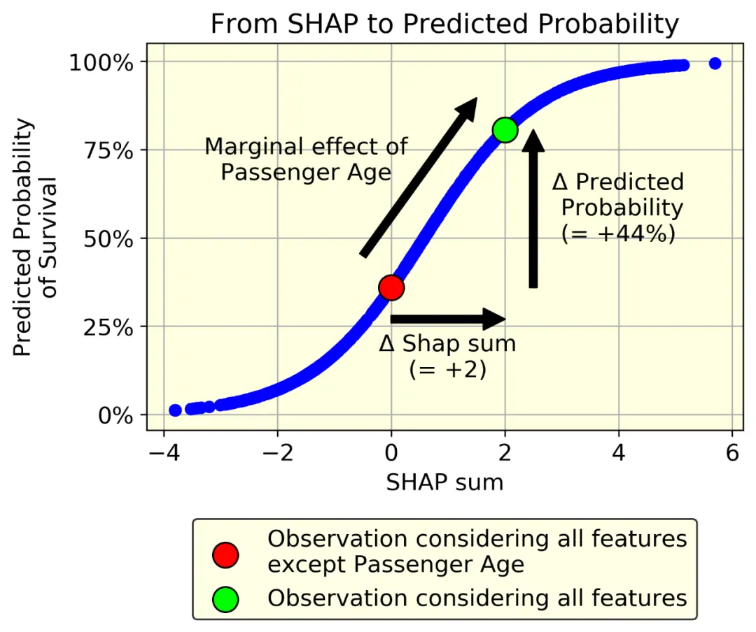
Take one individual. Suppose we know all variables except age, and their SHAP sum is 0. Now suppose age’s SHAP value is 2.

We only need the f() function to quantify age’s effect on predicted survival probability: f(2) − f(0). In our example, f(2) − f(0) = 80% − 36% = 44%.

Survival probability is undoubtedly easier to understand than raw SHAP values. Probability formula:

Final SHAP values per feature per sample:

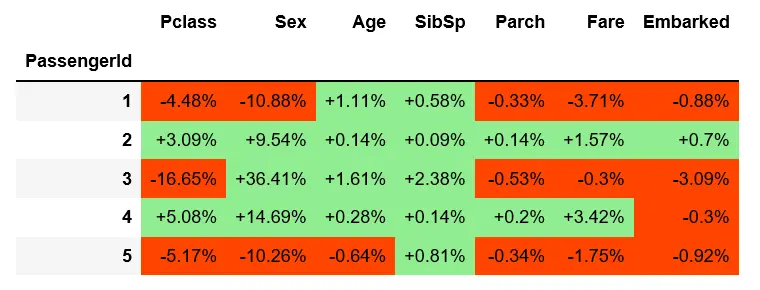
Why Do Probabilities Differ Across Samples for the Same Feature?

A third-class ticket lowers the first passenger’s survival probability by 4.48% (equivalent to −0.36 SHAP). Passengers 3 and 5 are also in third class. Because of interactions with other features, their impact on probability differs (−16.65% and −5.17% respectively).

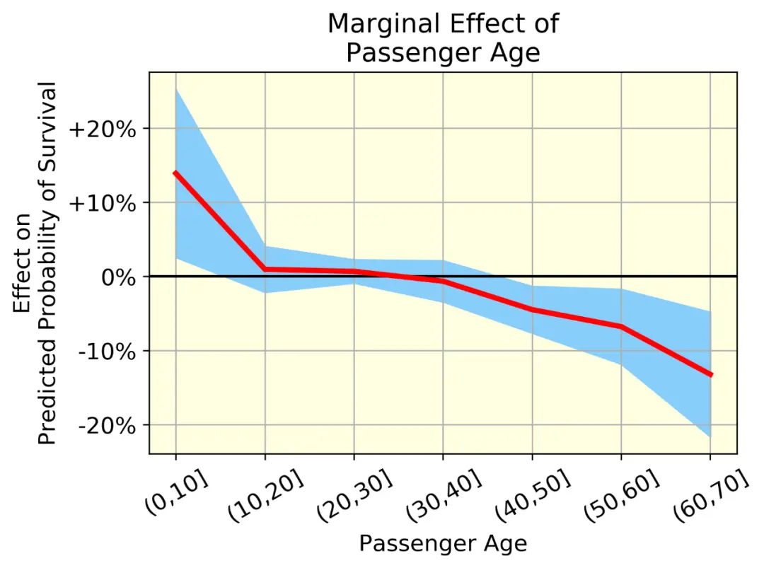
Analyze a single feature across multiple samples: effect of age on survival.

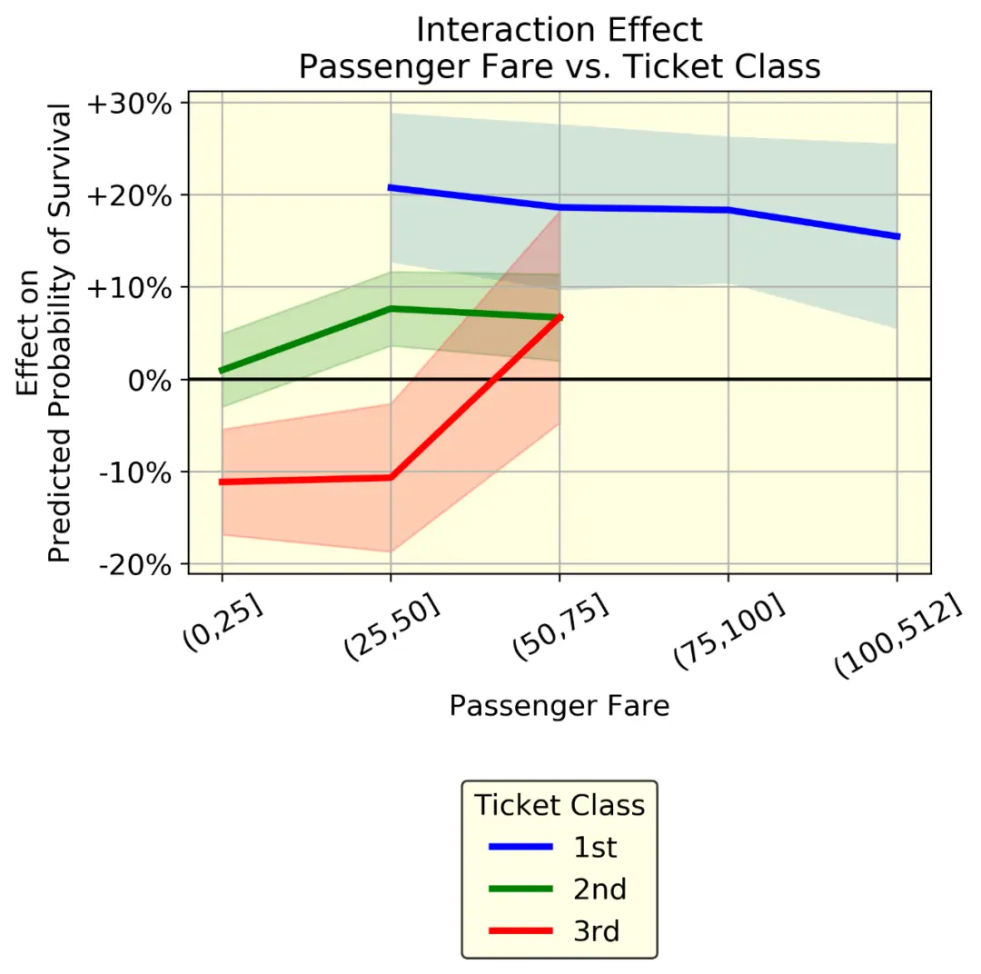
Analyze two features across multiple samples: fare and cabin class on survival.

Conclusions:

• We can quantify effects with probabilities instead of SHAP values. For example, on average, people aged 60–70 have 27% lower survival than those aged 0–10 (from +14% to −13%).
• We can visualize nonlinear effects. For fare, survival probability rises to a point, then dips slightly.
• We can show interactions. For fare and cabin class: if there were no interaction, the three lines would be parallel. Instead they behave differently. The blue line (first class) has slightly lower fare. The red line (third class) is especially interesting: among two third-class passengers, paying £50–75 yields higher survival than paying £50 (−10% to +5%).

Project URL