Writing
Machine Learning (9) — SVM Mathematical Foundations
Optimization, Lagrange multipliers, KKT conditions, distance to hyperplanes, and the perceptron model for SVM.
Support vector machines rely on many formulas and theorems; mastering them helps understand the algorithm.
Optimization problems
Optimization finds the global minimum of a function on a domain. Common cases (solutions may be local unless the function is convex):
(1)Unconstrained: gradient descent, Newton’s method, coordinate descent (gradient descent covered earlier);
(2)Equality constraints: Lagrange multipliers;
(3)Inequality constraints: KKT conditions.
Lagrange multipliers
Lagrange multipliers appear in constrained optimization. Parameter α is the multiplier (α ≠ 0).
2D example:

Equivalent to optimizing:

Geometric meaning: plot contours of f. Constraint g = c is one curve (red). At optimum, g = c is tangent to a contour f = d₁—gradients of f and g are parallel at the tangency point.
At zero gradient:

Partial derivatives:


Solve for x, y, λ; substitute into f for the extremum.
Example: minimize
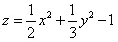
subject to

Code:
import numpy as np
import matplotlib as mpl
import matplotlib.pyplot as plt
import math
from mpl_toolkits.mplot3d import Axes3D
# Chinese display (original notebook)
mpl.rcParams['font.sans-serif'] = [u'SimHei']
mpl.rcParams['axes.unicode_minus'] = False
# Lagrange multiplier illustration
def f(x, y):
    return x**2 / 2.0 + y**2 / 3.0 - 1

# Build data
X1 = np.arange(-8, 8, 0.2)
X2 = np.arange(-8, 8, 0.2)
X1, X2 = np.meshgrid(X1, X2)
Y = np.array(list(map(lambda t: f(t[0], t[1]), zip(X1.flatten(), X2.flatten()))))
Y.shape = X1.shape

# Constraint
X3 = np.arange(-4, 4, 0.2)
X3.shape = 1,-1
X4 = np.array(list(map(lambda t: t ** 2+1, X3)))

# Plot
fig = plt.figure(facecolor='w')
ax = Axes3D(fig)
ax.plot_surface(X1, X2, Y, rstride=1, cstride=1, cmap=plt.cm.jet)
ax.plot(X3, X4 , 'ro--', linewidth=2)

ax.set_title(u'拉格朗日乘子的理解')
ax.set_xlabel('x')
ax.set_zlabel('z')
ax.set_ylabel('y')
plt.show()
Output:
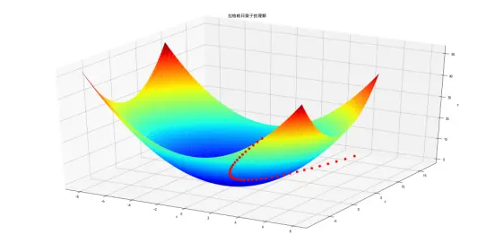
Understanding Lagrange multipliers helps with KKT below.
KKT conditions
Convex optimization with equalities and inequalities. Constraints reduce to equalities (= 0) and inequalities (≤ 0).
2D problem with an extra inequality:


Optimize:

Two cases:
(1)Feasible point strictly inside: set β = 0 to drop the constraint.
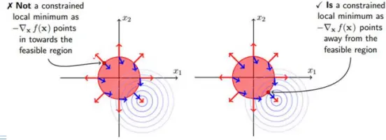
(2)On the boundary: if β ≠ 0, the solution lies on the boundary; the negative gradient of f should point away from the feasible region, aligned with ∇g—so β > 0.
Constraints:


Figure:
Since:
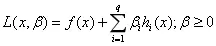

We get:
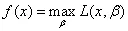

This is the dual problem. Brief dual properties:
Linear programs have duals; quadratics are QP; nonlinear → nonlinear optimization. Every LP has a dual.
(1)Dual of the dual is the primal;
(2)Dual is convex even if primal is not;
(3)Dual gives a lower bound on the primal;
(4)Under conditions, primal and dual solutions coincide.
Primal becomes:

This simplifies SVM training later.
Reference: Statistical Learning Methods (Li Hang), p.103.
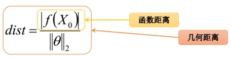
Distance from point to hyperplane
In 2D, point-to-line distance:
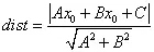
In higher dimensions:
Hyperplane:
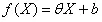
Distance:
Perceptron model
One of the oldest classifiers—simple, weak generalization, but foundation for SVM, neural nets, deep learning. Find a line or hyperplane separating classes.
Example: boys vs girls in a class—find a line (or hyperplane in high D) separating two classes. Assumption: linear separability.
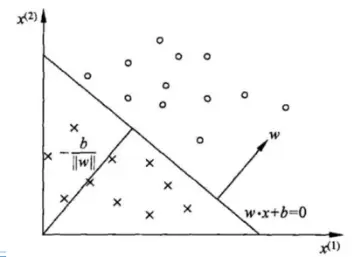
m samples, n features, binary labels:

Find hyperplane:

One class:

Other class:

Perceptron:
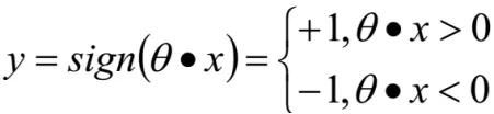
If correct:

If wrong:

Loss: sum of distances of misclassified points to the hyperplane:
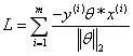
Scale ambiguity in numerator/denominator—fix denominator to 1 and minimize numerator (misclassification count proxy):
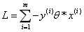
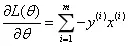
Gradient descent applies, but m is the misclassified set (changes each step)—use SGD or mini-batch, not full BGD. Perceptron typically uses SGD.