Machine Learning (8) — Other Clustering Methods

Hierarchical clustering

Following the previous chapter, this covers clustering ideas different from K-Means.

K-Means is convenient but struggles with choosing k and initial centers. Hierarchical clustering avoids some of that: cluster layer by layer—top-down (divisive) or bottom-up (agglomerative). Agglomerative bottom-up is most common.

Topics:

• Hierarchical clustering

• BIRCH

Hierarchical clustering

Hierarchical methods decompose a dataset until a condition holds. Two families: divisive and agglomerative.

Divisive hierarchical clustering

DIANA (Divisive Analysis) is top-down: all objects in one cluster, split by a rule (e.g. largest Euclidean distance) until cluster count or distance threshold.

Steps:

（1）Start with all samples in one cluster;

（2）In cluster c, find farthest pair a, b;

（3）Put a, b in separate clusters c1, c2;

（4）Assign remaining points in c by distance to a vs b (if dis(a)…

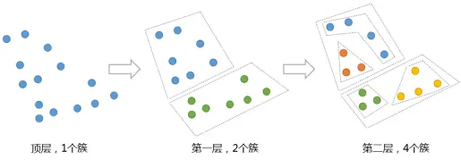
Top-down idea

Hierarchical K-means is a common top-down variant. Note: the red ellipse may be a better cluster, but orange and green split early in K-means and never merge again.

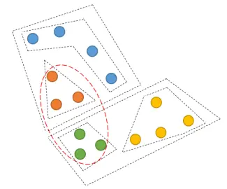
Using nearest point between clusters as inter-cluster distance is noise-sensitive and can yield elongated clusters.

Agglomerative hierarchical clustering

AGNES (Agglomerative Nesting) is bottom-up: each point is a cluster, merge stepwise; inter-cluster distance often from nearest points in different clusters until desired k.

Steps:

（1）Each sample is its own cluster;

（2）Compute inter-cluster distance (see below); merge closest c1, c2;

（3）Repeat until k clusters or stop condition.

(Illustration as in divisive section.)

8.1.1 Inter-cluster distance

For clusters C₁ and C₂, three linkages:

（1）Single link

Minimum distance between clusters:

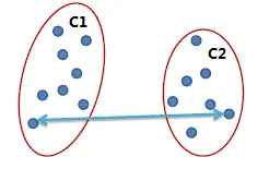
Single-link diagram

Nearest points define distance—noise-sensitive, chain-like clusters.

（2）Complete link

Maximum distance:

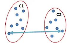
Farthest pair—tighter, compact clusters.

（3）Average link

Mean pairwise distance—reduces noise impact.

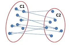
Hierarchical clustering summary

Pros and cons:

（1）Simple, intuitive

（2）Merge/split choice can be hard

（3）No undo of merges/splits

（4）Poor on very large data

（5）O(t·n²) time, t iterations, n points

Hierarchical clustering example

Agglomerative algorithm

Data:

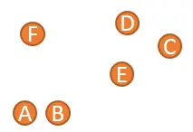
Points A–F → 6 clusters;

Single link: A and B closest → merge {A,B}; five clusters {A,B}, {C}, {D}, {E}, {F}:

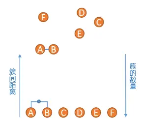
2. Repeat: merge closest pairs (same step as above in source);

3. {C} and {D} merge, then {C,D} with {E}, etc., until one cluster:

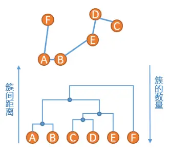
4. Cut dendrogram at threshold (red dashed line) → two clusters {A,B,C,D,E} and {F}:

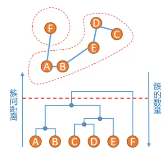
Agglomerative shows hierarchy at multiple scales; like hierarchical K-means, early splits cannot be undone; slow and memory-heavy on large n. BIRCH scales better.

BIRCH algorithm

BIRCH (Balanced Iterative Reducing and Clustering using Hierarchies): cluster features as 3-tuples; build a CF-tree with branching factor and cluster diameter limits; dynamic updates.

Steps:

（1）Build CF-tree; each node = cluster summary (count, linear sum, sum of squares);

（2）From root, descend to nearest child;

（3）At leaf, try to absorb point into nearest CF:

a) Yes → update CF

b) No → new CF; if leaf full, split farthest CF pair, reassign;

（4）Update non-leaf CF up to root.

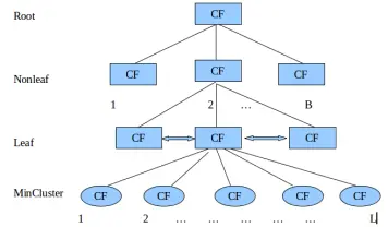
Example

Simulated data with sklearn Birch; compare parameters.

• Imports

# Import data, evaluation, clustering, plotting

from itertools import cycle
from time import time
import numpy as np
import matplotlib as mpl
import matplotlib.pyplot as plt
import matplotlib.colors as colors
from sklearn.preprocessing import StandardScaler
from sklearn.cluster import Birch
from sklearn.datasets.samples_generator import make_blobs

• Data

# 3 blobs, 100k samples, 2 features

## Avoid garbled Chinese in plots  mpl.rcParams['font.sans-serif'] = [u'SimHei']
mpl.rcParams['axes.unicode_minus'] = False
## Simulated data
xx = np.linspace(-22, 22, 10)
yy = np.linspace(-22, 22, 10)
xx, yy = np.meshgrid(xx, yy)
n_centres = np.hstack((np.ravel(xx)[:, np.newaxis],
np.ravel(yy)[:, np.newaxis]))
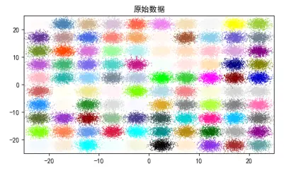
 # 100k samples, 2 features, 100 centers, Gaussian
 X, y = make_blobs(n_samples=100000, n_features=2, centers=n_centres, random_state=28)

Original data:

• Models

birch_models = [
    Birch(threshold=1.7, n_clusters=100),
    Birch(threshold=1.7, n_clusters=None)
]
# threshold: cluster diameter; branching_factor: max children

final_step = [ u'直径=1.7;n_clusters=100',
               u'直径=1.7;n_clusters=None'
               ]

plt.figure(figsize=(12, 8), facecolor='w')
plt.subplots_adjust(left=0.02, right=0.98, bottom=0.1, top=0.9)
colors_ = cycle(colors.cnames.keys())
cm = mpl.colors.ListedColormap(colors.cnames.keys())

5. Fit

for ind, (birch_model, info) in enumerate(zip(birch_models, final_step)):
    t = time()
    birch_model.fit(X)
    time_ = time() - t
    labels = birch_model.labels_
    centroids = birch_model.subcluster_centers_
    n_clusters = len(np.unique(centroids))
    print("Birch算法，参数信息为：%s；模型构建消耗时间为:%.3f秒；聚类中心数目:%d" % (info, time_, len(np.unique(labels))))

• Plot

    subinx = 221 + ind
    plt.subplot(subinx)
    for this_centroid, k, col in zip(centroids, range(n_clusters), colors_):
        mask = labels == k
        plt.plot(X[mask, 0], X[mask, 1], 'w', markerfacecolor=col, marker='.')
        if birch_model.n_clusters is None:
            plt.plot(this_centroid[0], this_centroid[1], '*', markerfacecolor=col, markeredgecolor='k', markersize=2)
    plt.ylim([-25, 25])
    plt.xlim([-25, 25])
    plt.title(u'Birch算法%s，耗时%.3fs' % (info, time_))
    plt.grid(False)

Original data subplot

plt.subplot(224)
plt.scatter(X[:, 0], X[:, 1], c=y, s=1, cmap=cm, edgecolors='none')
plt.ylim([-25, 25])
plt.xlim([-25, 25])
plt.title(u'原始数据')
plt.grid(False)
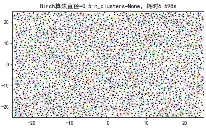
plt.show()

• threshold=0.5, n_clusters=100 vs None:

Birch算法，参数信息为：直径=0.5;n_clusters=100；模型构建消耗时间为:6.762秒；聚类中心数目:100

Birch算法，参数信息为：直径=0.5;n_clusters=None；模型构建消耗时间为:6.698秒；聚类中心数目:3205

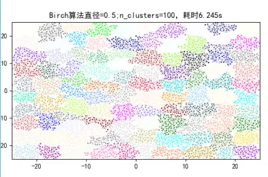
• threshold=1.7:

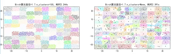
Birch算法，参数信息为：直径=1.7;n_clusters=100；模型构建消耗时间为:2.244秒；聚类中心数目:100

Birch算法，参数信息为：直径=1.7;n_clusters=None；模型构建消耗时间为:2.391秒；聚类中心数目:171

BIRCH vs agglomerative:

（1）Can revise structure (no permanent early split lock-in like agglomerative);

（2）CF-tree stores summaries, not all raw data—less memory;

（3）One pass over data vs per-iteration full scan;

（4）Streaming-friendly—no need for all data upfront.

Summary

Hierarchical clustering—especially agglomerative and BIRCH. Implementations use scikit-learn; spectral clustering, Apriori, etc. also exist. Master the ideas to compare methods.