Writing

Machine Learning (7) — Clustering Algorithms

Unsupervised clustering: distance metrics, K-Means, improvements, density clustering, and evaluation.

Clustering algorithms

Previous chapters covered supervised methods. This chapter introduces unsupervised learning—clustering. There is no target label “y”; we partition data by internal structure so within-cluster samples are similar.

Different clustering ideas yield different algorithms. This chapter covers three main ideas and their algorithms.

Topics:

“Distance”
K-Means
K-Means variants
Density clustering

Algorithm idea: “birds of a feather flock together”

We introduce similarity and basic similarity measures.

Algorithm idea

“Birds of a feather flock together.” Classification appears everywhere in nature and society—a class is a set of similar elements. Parents teach categories with cards: “This is a car.” “This is a plane.” “This is a fish.” “This is a bird.” “This is a circle.” “This is a rectangle.” Science often discovers new things and names classes. Categories we know come from common sense; for computers and clustering, algorithms group similar data. Our task: partition data into categories with minimal between-category similarity.

Partitioning by similarity

Compute pairwise similarity; group high-similarity samples. Common measures:

Minkowski distance (norm distance). p=1: Manhattan (2D example):

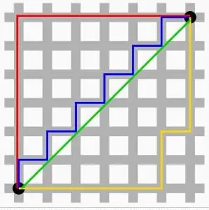
Manhattan distance

p=2: Euclidean:

p→∞: Chebyshev:

Euclidean is most common; Chebyshev when data are flattened.

Cosine similarity

Two features → cosine:

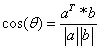
Common for text: bag-of-words vectors, cosine similarity—effective in practice.

Jaccard coefficient — for binary (0,1) features:

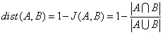
In item-based collaborative filtering, Jaccard improves on cosine when user ratings alone miss other signal—good for sparse data.

Clusters

ML names a category a cluster. Splitting M samples into k clusters requires k

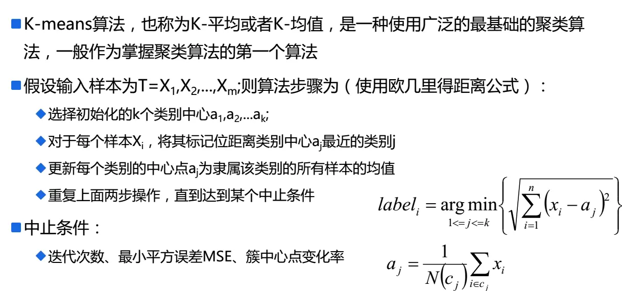
K-Means procedure

Illustrated:

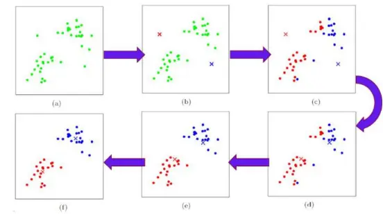
K-Means illustrated

In words and formulas:

N samples; choose two centers manually.
Distance from each sample to each center (often Euclidean, §9.1):

Split into two clusters; new centers = cluster means:

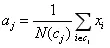
Repeat until stop condition. ### 8.1.1 K-Means loss

Minimize sum of distances to centers. Per-sample distance:

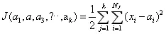
Minimize loss; partial derivatives give center update:

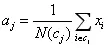
K-Means issues

Two major issues:

K-Means uses the mean as centroid; outliers skew the mean. Example: cluster {2,4,6,8,100} → mean 24, far from most points; median 6 (K-Medoids) may be better.

Initialization sensitivity

K-Means depends on initial centers. Fix: multiple random inits and pick best, or better init (below). Example: four obvious regions:

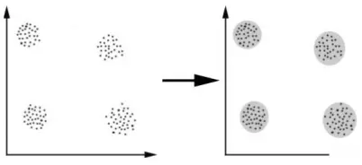
Clustering dataset

Random centers A,B,C,D:

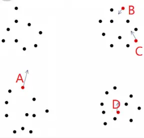
K-Means result:

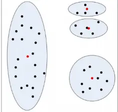
K-Means example

Use sklearn simulated data; K-Means clustering and centers.

Build data

Gaussian blobs, 4 clusters, 1000 samples:

from sklearn.datasets import make_blobs
N = 1000
centers = 4

Two features:

X, Y = make_blobs(n_samples=N, n_features=2, centers=centers, random_state=0)

Model

from sklearn.cluster import KMeans

Specify k, max iterations, or center change threshold.

km = KMeans(n_clusters=centers, init='random', random_state=28)

km.fit(X)

Predict

y_hat = km.predict(X)

Centers and inertia (loss)

print("所有样本距离所属簇中心点的总距离和为:%.5f" % km.inertia_)  print("所有的中心点聚类中心坐标:")  cluter_centers = km.cluster_centers_  print(cluter_centers)  print("score其实就是所有样本点离所属簇中心点距离和的相反数:")  print(km.score(X))

Output:

所有样本距离所属簇中心点的总距离和为:1764.19457

所有的中心点聚类中心坐标:

[[-6.32351035  7.09545595]

 [-7.51888142 -2.01003574]

 [ 6.0528514   0.24636947]

 [ 4.26881816  1.08317321]]

score其实就是所有样本点离所属簇中心点距离和的相反数:

-1764.19457007324

Plot

import matplotlib.pyplot as plt  import matplotlib as mpl

cm = mpl.colors.ListedColormap(list('rgby'))  plt.figure(figsize=(15, 9), facecolor='w')  plt.subplot(121)  plt.title(u'原始数据')  plt.grid(True)  plt.scatter(X[:, 0], X[:, 1], c=Y, s=30, cmap=cm, edgecolors='none')  plt.subplot(122)  plt.scatter(X[:, 0], X[:, 1], c=y_hat, s=30, cmap=cm, edgecolors='none')  plt.title(u'K-Means算法聚类结果')  plt.grid(True)  plt.show()

Result:

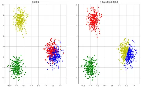
Original vs K-Means

With k=3 and k=5:

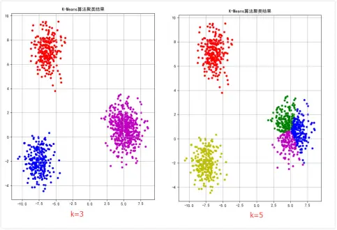
K-Means with different k

K-Means improvements

K-Means is simple and widely used, but k must be chosen and init matters. Variants below.

K-Means++

Init centers as far apart as possible to reduce bad random starts. Steps:

q Pick one point as first center

q For each x, compute D(x) = sum of distances to existing centers; pick next center with probability proportional to D(x)²

q Repeat until k centers

Works well unless data are very scattered.

Reference: Bahman Bahmani, Benjamin Moseley, Andrea Vattani. Scalable K-Means++.

K-Means||

k-means++ is sequential (k passes)—hard to parallelize on huge data.

K-Means|| samples k points per round, repeat O(k log n) times, cluster those k points, use as K-Means init. Often a few rounds suffice.

Bisecting K-Means

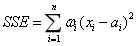
Another init fix: start with one cluster, bisect one cluster (largest SSE or largest cluster) repeatedly until k clusters.

Steps:

q Start with all samples in one cluster

q Bisect one cluster with K-Means into two; add to queue

q Repeat until stop (cluster count, SSE, iterations)

q Queue holds final clusters

Split rule:

（1）Pick cluster with largest SSE:

（2）Split largest cluster by size

Canopy algorithm

Canopy (2000), popular with Hadoop, pre-clusters for algorithms like k-means—reduces distance computations.

（1）Samples L=x₁…xₘ, thresholds T₁, T₂ (T₁>T₂)

（2）Take P from L; distance to all canopy centers (first point starts a canopy); min distance D(P,aⱼ)

（3）If D < T₁, add P to that canopy

（4）If D < T₂, also recompute center, remove P from L

（5）If D > T₁, P starts new canopy

（6）Repeat until L stable or empty

Flowchart:

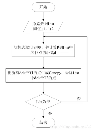
Canopy flowchart

Canopies may overlap; every point belongs to some canopy. Canopy + k-means: T₁, T₂ critical—too large T₁ → too many iterations/canopies; too small → poor accuracy.

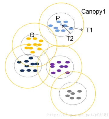
Canopy illustration

Mini Batch K-Means

Uses mini-batches instead of full data each step—faster, slightly less accurate; good for huge datasets. Same idea as mini-batch SGD.

（1）Sample subset; K-Means for k centers

（2）Sample more points; assign to nearest center

（3）Update centers

（4）Repeat until stable

Similar use cases to K-Means; below we compare speed.

8.1.1 Clustering evaluation

Supervised metrics: accuracy, precision, recall. Unsupervised: clusters need not match labels unless distribution aligns or within-cluster similarity > between-cluster.

Common metrics:

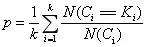
Homogeneity (completeness) — one cluster, one true class; homogeneity ≈ per-cluster purity:

Rand index (RI)

Given true labels C, clustering K; a = pairs same in both, b = pairs different in both:

Numerator: agreeing pairs. Denominator: all pairs. RI ∈ [0,1]; higher is better. Random clustering may not be ~0; Adjusted Rand Index (ARI):

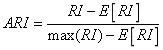
ARI ∈ [-1,1]; higher = better agreement.

Pros: (1) random ARI ≈ 0; (2) [-1,1]; (3) compare algorithms. Cons: needs true labels.

Silhouette coefficient

No labels needed.

a = mean intra-cluster distance for i (smaller → i fits cluster). b = min mean distance to other clusters (larger → i not in those). Silhouette s:

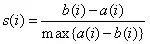
s near 1: good; near -1: wrong cluster; ~0: boundary. sklearn: metrics.silhouette_score.

from sklearn import metrics  from sklearn.metrics import pairwise_distances
from sklearn import datasets
dataset = datasets.load_iris()
X = dataset.data
 y = dataset.target
import numpy as np
from sklearn.cluster import KMeans
kmeans_model = KMeans(n_clusters=3, random_state=1).fit(X)
labels = kmeans_model.labels_
metrics.silhouette_score(X, labels, metric='euclidean')

Output:

兰德系数为：

0.5730973570083832

Example: Mini Batch K-Means vs K-Means

Compare speed on larger data; evaluate with metrics above.

API: http://scikit-learn.org/0.19/modules/generated/sklearn.cluster.KMeans.html#sklearn.cluster.KMeans

# n_clusters, init, n_init (multiple inits), max_iter

sklearn.cluster.KMeans(n_clusters=8, init='k-means++', n_init=10, max_iter=300) [](#sklearn.cluster.MiniBatchKMeans "Permalink to this definition")

1. Imports

import time  import numpy as np  import matplotlib.pyplot as plt  import matplotlib as mpl  from sklearn.cluster import MiniBatchKMeans, KMeans  from sklearn.metrics.pairwise import pairwise_distances_argmin  from sklearn.datasets.samples_generator import make_blobs

2. Data

# 3 blobs, 3000 samples, 2 features

# centers = [[1, 1], [-1, -1], [1, -1]]  clusters = len(centers)  # k=3  # X, Y = make_blobs(n_samples=3000, centers=centers, cluster_std=0.7, random_state=0)

3. Models

k_means = KMeans(init='k-means++', n_clusters=clusters, random_state=28)  t0 = time.time()  k_means.fit(X)  km_batch = time.time() - t0  print ("K-Means算法模型训练消耗时间:%.4fs" % km_batch)

batch_size = 100  mbk = MiniBatchKMeans(init='k-means++', n_clusters=clusters, batch_size=batch_size, random_state=28)  t0 = time.time()  mbk.fit(X)  mbk_batch = time.time() - t0  print ("Mini Batch K-Means算法模型训练消耗时间:%.4fs" % mbk_batch)

# Output:

L- Means算法模型训练消耗时间:0.0416s

M- Mini Batch K-Means算法模型训练消耗时间:0.0150s

4. Predict

km_y_hat = k_means.predict(X)  mbkm_y_hat = mbk.predict(X)  print(km_y_hat[:10])  print(mbkm_y_hat[:10])  print(k_means.cluster_centers_)  print(mbk.cluster_centers_)

# Output:

[0 1 0 2 1 1 1 1 2 1]

[[-1.07159013 -1.00648645]

 [ 0.96700708  1.01837274]

 [ 1.07705469 -1.06730994]]

[[ 1.02538969 -1.08781328]

 [-1.06046903 -1.01509453]

 [ 0.97734743  1.08610316]]

5. Sort centers

k_means_cluster_centers = k_means.cluster_centers_  mbk_means_cluster_centers = mbk.cluster_centers_  print ("K-Means算法聚类中心点:\ncenter=", k_means_cluster_centers)  print ("Mini Batch K-Means算法聚类中心点:\ncenter=", mbk_means_cluster_centers)  order = pairwise_distances_argmin(k_means_cluster_centers,                                    mbk_means_cluster_centers)

K-Means centers:

center= [[-1.07159013 -1.00648645]

 [ 0.96700708  1.01837274]

 [ 1.07705469 -1.06730994]]

### Mini Batch K-Means centers:

center= [[ 1.02538969 -1.08781328]

 [-1.06046903 -1.01509453]

 [ 0.97734743  1.08610316]]

6–8. Plots and difference subplot (code as in source)

different = list(map(lambda x: (x!=0) & (x!=1) & (x!=2), mbkm_y_hat))  for k in range(clusters):      different += ((km_y_hat == k) != (mbkm_y_hat == order[k]))  identic = np.logical_not(different)  different_nodes = len(list(filter(lambda x:x, different)))  plt.subplot(224)  plt.plot(X[identic, 0], X[identic, 1], 'w', markerfacecolor='#bbbbbb', marker='.')  plt.plot(X[different, 0], X[different, 1], 'w', markerfacecolor='m', marker='.')  plt.title(u'Mini Batch K-Means和K-Means算法预测结果不同的点')  plt.xticks(())  plt.yticks(())  plt.text(-3.8, 2,  'different nodes: %d' % (different_nodes))  plt.show()

Output:

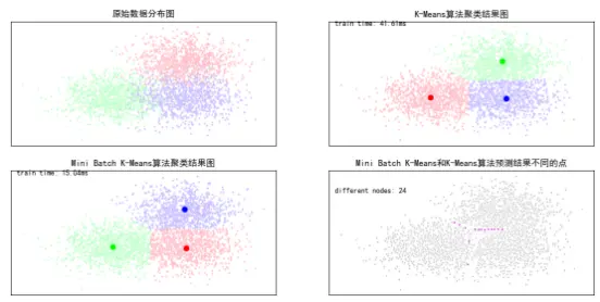
Comparison

Mini Batch is more than 2× faster with similar quality.

Non-convex data (below) breaks K-Means; need other methods (next chapter).

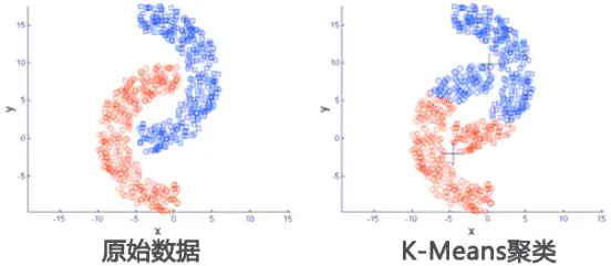
Non-convex clustering

Chapter summary

K-Means and variants for unsupervised clustering via clusters. We covered workflow, init sensitivity, and Mini Batch for scale. When K-Means fails, other ideas follow in the next chapter.