Writing
Machine Learning (6) — Decision Trees
Preface: decision trees build a tree model first, then derive the loss function as a metric; information entropy, pruning, and visualization.
Preface
Earlier chapters covered the workflow for building regression models. Machine learning aims to find the target function, optimize it, and minimize it at each iteration—the optimal solution is the model parameters when the objective is smallest. This chapter introduces a model whose workflow is the opposite of regression: the decision tree. After building the tree model, we obtain the loss function, which becomes the metric for evaluating the tree. When features are numerous and large, this intuitive tree structure can split features first, then build the model.
Topics in this chapter:
-
Information entropy
-
Decision trees
-
Decision tree optimization
-
Tree pruning
-
Decision tree visualization
Algorithm idea: from decisions to decision trees
This section starts from everyday decision-making to introduce the basic idea of decision trees, then defines key concepts.
Decisions
What is a decision? In life we often rely on information to decide—choosing a university, a major, a job, a partner… Or when you go home for the holidays you might hear:
Mother: I want to introduce you to someone.

You: How old are they?

Mother: 26.

You: Are they good-looking?

Mother: Quite handsome.

You: Where do they work?

Mother: Same city as you.

You: What do they do?

Mother: I heard they're a programmer.

You: OK, I'll meet them.
Here you used the core idea of a decision tree: from many features of the “candidate,” you decide meet or don’t meet.
That process helps us understand tree construction. Computers predict from data. A more intuitive example:
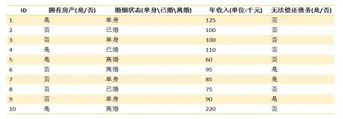
Debt repayment table
Given 10 samples, build a decision tree to judge whether debt can be repaid.
The decision tree from the data:
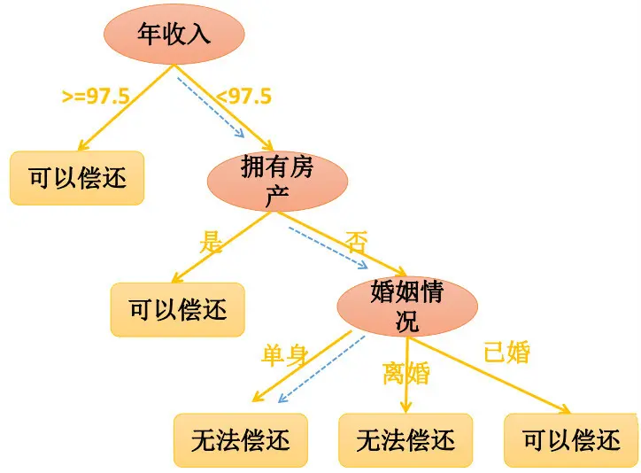
Debt repayment decision tree
Red nodes (root/internal) are split conditions; orange nodes (leaves) are decisions. Building a tree from data is tree construction. Note: finding the best root and optimizing leaves is the main task of decision tree algorithms.
Decision tree
- Definition
Based on the above:
A decision tree analyzes situations given occurrence probabilities; it is an intuitive probabilistic diagram. It is a predictive model mapping object attributes to values; a tree where each internal node tests an attribute, each branch is a test outcome, and each leaf is a class. Decision trees are very common supervised classification algorithms.
Note: “internal node” and “leaf node.” Prediction starts at the root, tests features, follows branches by value, until a leaf gives the class. Trees split into classification trees (discrete labels) and regression trees (continuous targets), with algorithms such as ID3, C4.5, and CART.
- Tree construction
The focus is attribute selection and topology. Key step: split attributes so child subsets are as pure as possible (items in a split belong to the same class). Note: find split attributes and make leaves “purer.” Steps:
q 1. Treat every feature as a node candidate;

q 2. For each feature and each split, find the best split; partition into child nodes N1, N2, …, Nm; compute purity after the split;

q 3. Choose the best feature and split; obtain final children N1, N2, …, Nm;

q 4. Recurse on N1…Nm until each leaf is sufficiently pure.- Attribute types
When building the tree, handle attribute types differently:
q Discrete attributes, non-binary tree: one branch per attribute value
q Discrete attributes, binary tree required: test membership in a subset—"in subset" vs "not in subset"
q Continuous attributes: pick a split point; branches for > split point and <= split point
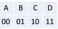
Encoding diagram
Each letter uses 2 bits on average.
Encoding the sequence as in the figure below: 010001100111000
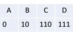
Encoding diagram 2
Average bits per symbol:

Encoding formula
This closely resembles Shannon entropy.
### Information entropy
Also called Shannon entropy (Shannon, 1948): a more ordered system has lower entropy; a more chaotic system has higher entropy. Entropy measures order.
1. **Information content**
Information in a sample: if an event is very likely, it carries little information. For example:
" The sun rises in the east" is certain and carries no information.
" I ran into Jay Chou while shopping yesterday" carries a lot of information.
2. **Entropy**
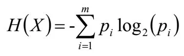
The entropy formula:
Information entropy formula
For m events in random variable X, average bits needed is entropy. If one event dominates, entropy drops. Example:
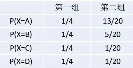
Eight horses in two groups, win probabilities:
Horse race information
Group 1: equal odds—hard to guess. Group 2: horse A likely wins. Entropy: group 1 H(X)=2; group 2 H(X)=1.336.
### Conditional entropy H(Y|X)
In essence, expected entropy.
1. **Definition**
Entropy of Y given X:
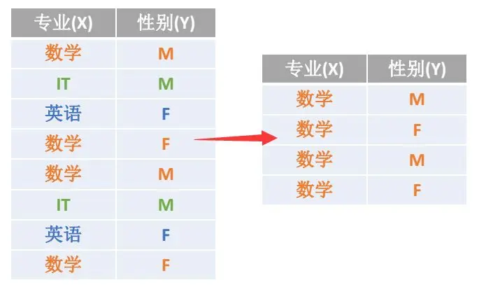
Example:
Major information
When X=math, H(Y|X=math)=1. Average over all x gives conditional entropy:

## Building the decision tree model
### Measuring purity
Question 1: We want splits that make leaves "pure"—how measure purity? Question 2: How choose splits? Answer: information gain.
1. **Information gain**
Lower entropy means one class dominates—a purer leaf. Entropy measures purity. After purity per attribute, pick the split with largest information gain (most purity gained). Formula: Gain = Δ = H(D) − H(D|A). Gain is empirical entropy of D minus conditional entropy given A. Other purity metrics: Gini index and error rate.
2. **Stopping criteria**
Recursion needs stop conditions:
q Stop when each child has only one class
q Stop when node count < threshold or max iterations; assign majority class P(i)
Method 1 can overfit. Method 2 is common.
3. **Evaluation**
Like other classifiers: accuracy, recall, F1. Uniquely, sum of leaf purities—lower sum means clearer splits:
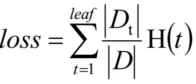
By the loss-function view, this is the loss or objective; we want the tree that minimizes it.
4. **Three classic algorithms**
q ID3
q C4.5
q CART
ID3 uses entropy and information gain; each step picks max gain. Fast and simple; weak with many features, ignores attribute relations, noise-sensitive—small data.
C4.5 uses gain ratio instead of gain, prunes, handles continuous attributes by discretization; picks max gain ratio. Formula context: P(i)=−∑P(i)log₂(P(i)).
Information gain ratio:
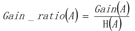
Higher accuracy, simple, no limit on feature count; slower than ID3.
CART uses binary trees; features can be reused—most common in practice (used in examples below).
5. **Classification vs regression trees**
Classification uses gain, gain ratio, or Gini; leaf prediction is majority class.
Regression leaves predict the mean; MSE is common:
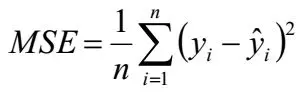
Usually CART for regression trees.
## Decision tree optimization
Two main approaches: pruning and random forest (forest covered in ensemble learning). Here: pruning.
### Pruning
Pruning is basic and useful; two types.
**1. Pre-pruning**
Stop early while building. Common rules:
-
Limit tree depth
-
Limit samples per leaf
**2. Post-pruning**

Build full tree, then prune:
-
Replace a subtree with one leaf (majority class);
-
Replace one subtree with another; post-pruning cost is computation.
Post-pruning (like cross-validation): start from full tree T₀, prune to T₁, T₂, … until root only; evaluate T₀…Tₖ on validation; pick best Tₐ (min loss).

For tree T₀:
1 Compute pruning coefficient for every internal non-leaf
2 Find minimum coefficient node; delete children → tree Tₖ
3 If several minima, prune the node with most samples
4 Repeat until one node remains
5 Obtain T₀, T₁, …, Tₖ
6 Pick best Tₐ on validation set
How compute pruning coefficient? Original loss:
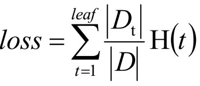
More leaves → more complex tree → higher loss. Add coefficient α on leaf count: loss = loss + α × leaf. Before prune loss(r), after loss(R). Require loss(r) − loss(R) = 0; then α = (loss(r) − loss(R)) / (leaf − 1). Use α for optimization.
## Decision tree visualization
Visualization helps inspect the model. It uses Graphviz. Setup:
### Install and configure
- Install Graphviz
q Download: http://www.graphviz.org/
q Run the installer (double-click .msi)
q Add bin folder to PATH
- Python packages
01 pip install graphviz
02 pip install pydotplus
### Example

Two approaches; assume model is trained:

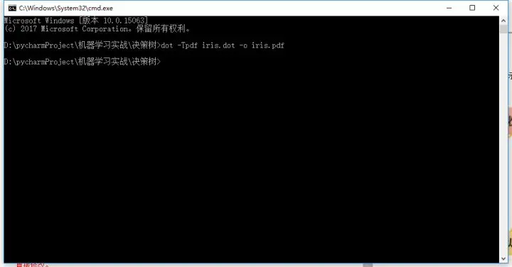
**1. Export to dot, convert via CLI: dot -Tpdf iris.dot -o iris.pdf**
01 /// Import visualization
02 from sklearn import tree
03 with open(‘model.dot’, ‘w’) as f:
04 da = tree.export_graphviz(tre, out_file=None)
05 f.write(da)
**Convert to PDF:**
2. **Display with Image object**
01 /// Import visualization
02 import pydotplus
03 from sklearn import tree
04 dot_data= tree.export_graphviz(model, out_file=None)
05 graph = pydotplus.graph_from_dot_data(dot_data)
06 Image(graph.create_png())
Note: “model” is the trained decision tree
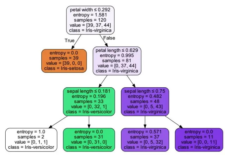
`tree.export_graphviz` accepts colors for nicer plots:
Decision tree visualization
Each node shows sample count, feature count, split attribute, etc.
## Full example
Using regression workflow steps and this chapter's theory: Iris dataset, build a tree, predict, visualize.
Note: Why Iris? Classic ML dataset in sklearn docs; it shows how depth affects overfitting.
### Workflow

**1. Collect and prepare data**

Download from http://archive.ics.uci.edu/ml/datasets/Iris

150 samples, 3 classes, 50 each, 4 features (sepal/petal length/width) → Setosa, Versicolour, Virginica.

- **Load data**
-
import pandas as pd
-
path = “datas/iris.data”
-
df = pd.read_csv(path,sep=”,“,header=None)
First five rows:
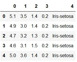
Iris data
- **Features and target**
First three columns are features; fourth is target.
-
x = df.iloc[:,0:4]
-
y = df.iloc[:,4]
-
** Split train and test**
from sklearn.model_selection import train_test_split
-
from sklearn.model_selection import train_test_split
-
x_train,x_test,y_train,y_test=train_test_split(x,y,test_size=0.2,random_state=0)
Why use a library? Concise code. Manual split example:
def loadDataset(fileName,split,trainingSet=[],textSet=[]):
with open(fileName, "r") as f:

    reader = csv.reader(f)

    data = list(reader)

    for x in range(len(data) - 1):

        for y in range(4):

            data[x][y] = float(data[x][y])

        if random.random()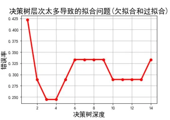
Effect of tree depth
Analysis: As depth increases, accuracy rises until a point (depth 6): train accuracy peaks while test accuracy falls—overfitting. Fix: limit depth (e.g. 2) or use many trees—random forest.
Chapter summary
Decision trees decide from raw data by splitting on features. The key is minimizing leaf entropy. We covered optimization, depth vs overfitting, and feature importance from splits. Next chapter addresses the question raised at the end.