Machine Learning (3) — Regression Models

Preface: Following the previous article, when predicted and true values differ greatly, this post covers using polynomial weights to improve fit (R²), remedies for overfitting, regularization terms L1 and L2, Ridge regression, and LASSO regression.

Objective Function

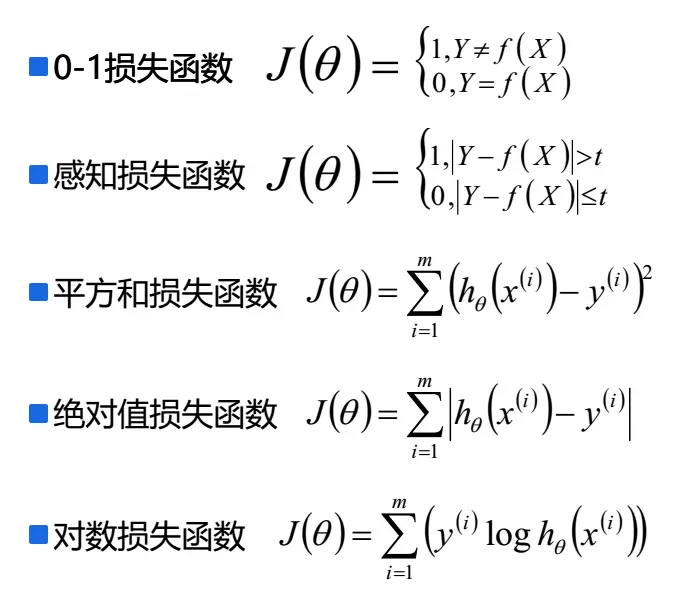
In machine learning, the objective function indicates the direction during model training (parameter estimation). For example, linear regression aims to minimize the objective function; it uses the sum-of-squares loss. Perceptron loss is used in SVM; log loss is used in logistic regression, and so on. Common objective functions:

Polynomial Expansion

• When a linear model cannot accurately fit the data, we expand the data. Here we perform polynomial expansion on top of a linear model, using curves to fit the data for a better model.

• Concept: combine features with each other to form new features—a process that mathematically maps low-dimensional data points to a higher-dimensional space. It is a kind of feature engineering. For univariate linear regression: 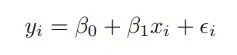Univariate polynomial regression becomes: As shown below, describing the model with a straight line yields large error, while polynomial expansion fits much better: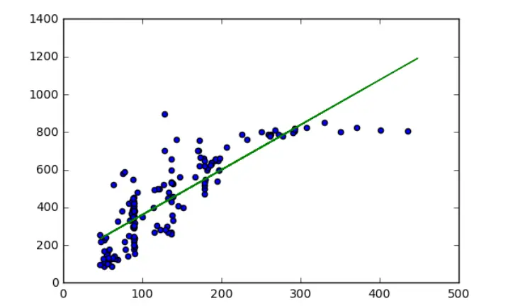 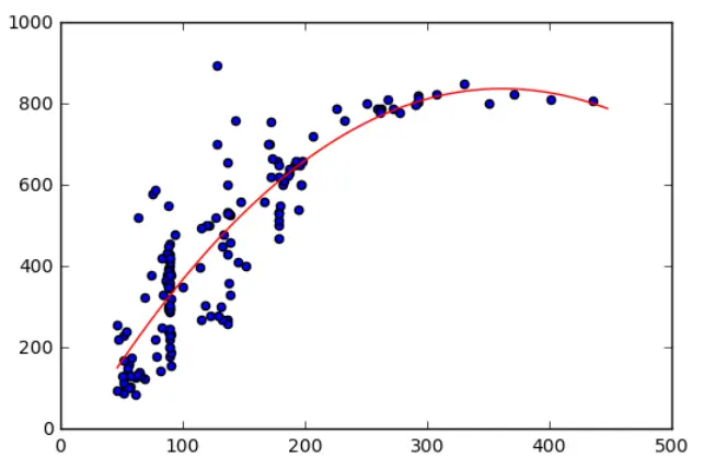We use polynomial expansion to improve the model from the previous article, introducing from sklearn.preprocessing import PolynomialFeatures. Improved code:

#-*- conding:utf-8 -*-
#准确率：print("电流预测准确率: ", lr2.score(X2_test,Y2_test))
from sklearn.model_selection import train_test_split
from sklearn.linear_model import LinearRegression
from sklearn.preprocessing import StandardScaler
from sklearn.preprocessing import PolynomialFeatures
import numpy as np
import pandas as pd
from pandas import DataFrame
import matplotlib as mpl
import matplotlib.pyplot as plt
import time
#防止中文乱码
mpl.rcParams['font.sans-serif']=[u'simHei']
mpl.rcParams['axes.unicode_minus']=False
#加载数据
path="household_power_consumption_1000.txt"
df = pd.read_csv(path,sep=";")
#数据处理，包括，清除空数据
df1=df.replace("?",np.nan)
data = df1.dropna(axis=0,how="any")
#把数据中的字符串转化为数字
def data_formate(x):
    t = time.strptime(' '.join(x), '%d/%m/%Y %H:%M:%S')
    return (t.tm_year, t.tm_mon, t.tm_mday, t.tm_hour, t.tm_min, t.tm_sec)
X = data.iloc[:,0:2]
x = X.apply(lambda x:pd.Series(data_formate(x)),axis=1)
y = data.iloc[:,4]
#数据分集
x_train,x_test,y_train,y_test=train_test_split(x,y,test_size=0.2,random_state=0)
#标准化
ss = StandardScaler()
x_train=ss.fit_transform(x_train)
x_test=ss.transform(x_test)
#模型训练
pol = PolynomialFeatures(degree = 9)
xtrain_pol = pol.fit_transform(x_train)
xtest_pol = pol.fit_transform(x_test)
lr = LinearRegression()
lr.fit(xtrain_pol,y_train)
y_pridect=lr.predict(xtest_pol)
#输出参数
print("模型的系数(θ):",lr.coef_)
print("模型的截距:",lr.intercept_)
# print("训练集上R2:",lr.score(x_train, y_train))
print("测试集上R2:",lr.score(xtest_pol, y_test))
mse = np.average((y_pridect-y_test)**2)
rmse = np.sqrt(mse)
print("rmse:",rmse)
#画图
t=np.arange(len(y_test))
plt.figure(facecolor='w')#建一个画布，facecolor是背景色
plt.plot(t, y_test, 'r-', linewidth=2, label='真实值')
plt.plot(t, y_pridect, 'g-', linewidth=2, label='预测值')
plt.legend(loc = 'upper left')#显示图例，设置图例的位置
plt.title("线性回归预测时间和电压之间的关系", fontsize=20)
plt.grid(b=True)#加网格
plt.show()

When degree = 1, 2, 3, 4, the plots look like this:

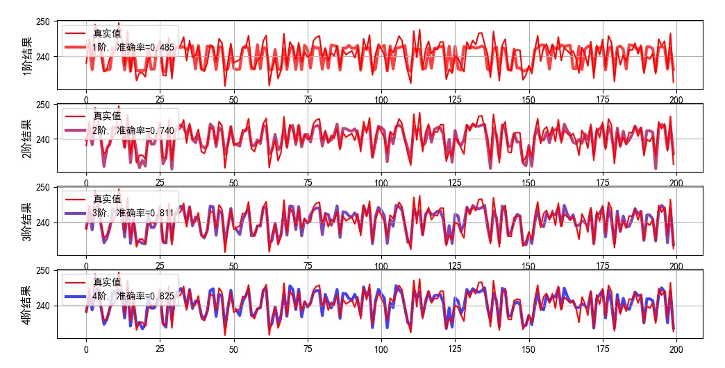
Accuracy improves considerably. When degree = 9, parameter values become abnormally large—this is overfitting. Model coefficients (θ): [ 1.75147911e+12 4.24195739e+10 -2.94579982e+11 … 0.00000000e+00

0.00000000e+00 0.00000000e+00]

To prevent overfitting we introduce the regularization norm.

Regularization

• L1-norm L2-norm The corresponding regression models are Ridge regression (L2-norm) and LASSO regression (L1-norm).

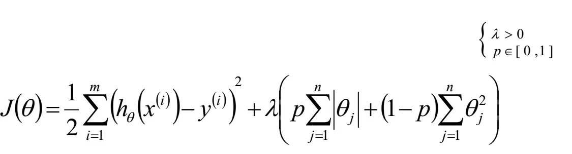
• ElasticNet algorithm: a linear regression model that uses both L1 and L2 regularization is called ElasticNet (elastic net).

Hyperparameter Tuning in Machine Learning

In practice, for various algorithm models (take elastic net as an example), solving for θ, λ, and ρ is usually handled by the library (the algorithm is already implemented). What developers mainly tune are λ and ρ—this process is called hyperparameter tuning.

• Cross-validation: split training data into several folds; use one fold for validation to find optimal hyperparameters λ and ρ—for example, 10-fold or 5-fold cross-validation (Scikit-learn default), etc.