Writing
Machine Learning (19) — Feature Engineering
Preface: feature engineering is central to machine learning and directly affects model quality.
Preface: feature engineering is central to machine learning and directly affects model quality.
Data Collection
Before machine learning, when collecting data we mainly follow these rules to find what we need:
-
What data does the business need? Based on business rules, find as many independent variables as possible that affect the target.
-
Data availability: consider acquisition cost; check whether data covers all cases and how trustworthy it is.
-
Data sources: user behavior logs; business data (products, users/members, …); third-party data (crawled, purchased, partner data, …).
-
Storage: model-building data usually lives on local disk, relational databases, or distributed platforms. Local disk, MySQL, Oracle, HBase, HDFS, Hive.
Data Cleaning
-
Preprocessing: choose tools (SQL or Python); inspect metadata (field definitions, sources) and sample rows manually to spot issues early.
-
Format and content errors: inconsistent date/time/number formats—normalize to one format, common when merging sources. Stray characters (spaces at start/middle/end)—semi-automated checks plus manual cleanup. Wrong content in a field (name in gender column, phone in ID field, etc.).
-
Remove unneeded data: we often collect broadly, but not every field helps the model—and more fields do not always mean better models; they slow training. Drop useless fields with backups of raw data.
-
Linkage validation: with multiple sources, verify links when merging—e.g. offline car purchase vs. phone survey linked by name and phone to confirm the same vehicle; adjust if not.
Imbalanced Data
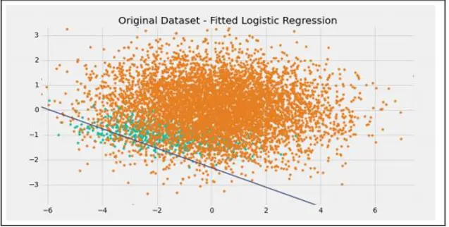
-
Set loss weights so misclassifying minority classes costs more than majority classes—parameters shift toward accurate minority prediction. Use scikit-learn
class_weight. -
Undersampling: randomly sample from the majority class to balance classes.
-
Synthetic oversampling: generate more samples—works in small-data settings. SMOTE is common; it creates new points from similar minority samples in feature space.
Feature Transformation
Feature transformation converts raw fields into algorithm-ready numeric input, including:
-
Text to numbers
-
Missing value imputation
-
One-hot encoding of categorical features
-
Binarization of quantitative features
-
Standardization and normalization
-
Text features: models require numeric input. Common methods: bag-of-words (BOW/TF), TF-IDF, HashingTF, Word2Vec (similarity).
-
Missing values: typical steps—define missing scope, drop unusable fields, fill values, re-fetch if needed. Filling is most important.
-
One-hot encoding (OneHotEncoder): for categorical data, use N bits for N states; only one bit active. Example:
['male','female']→ male [1,0], female [0,1]. Example:
#-*- conding:utf-8 -*-
'''
亚编码,先把特征转为数字,再进行亚编码处理
'''
import numpy as np
import matplotlib as mpl
import pandas as pd
import matplotlib.pyplot as plt
from sklearn.preprocessing import OneHotEncoder
path = "car.data"
data = pd.read_csv(path, header=None)
#查看数据
for i in range(7):
    print(np.unique(data[i]))
#将字符串转化为数字,用pd.Categorical
# pd.Categorical(data)
x=data.apply(lambda x:pd.Categorical(x).codes)
print(x.head(5))
#进行亚编码操作,toarray()方法转化为数组
en=OneHotEncoder()
x = en.fit_transform(x)
print(x.toarray())
print(en.n_values_)
#在进行转化
df=pd.DataFrame(x.toarray())
print(df.head(5))-
Binarization (Binarizer): for continuous quantitative features, threshold to 1 if above, 0 otherwise. Very common—split each feature at different thresholds, then combine. Can extend to multi-threshold binning.
-
Standardization (z-score): per feature column, use mean and variance to map values to standard normal:
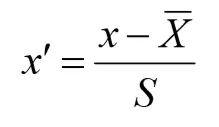
-
Min-max scaling: scale to a given interval:
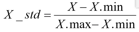
-
Normalization (regularization): unlike standardization, operates row-wise to make each row a “unit vector”; L2 formula:
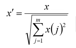
-
Comparison: standardization reduces impact of different feature scales—outliers and wide ranges can mislead models or bias gradient-based training toward large-scale features. Reshaping distributions helps (1) faster convergence and (2) better precision. Normalization (min-max) makes dimensions comparable without changing distribution shape (same-type features stay same-type). Regularization constrains features via norms, reducing overfitting like L1/L2 in ML; it does not change distribution but alters feature correlations. Broadly, standardization, min-max, and normalization overlap; some texts call standardization + min-max “standardization” and normalization “归一化.” In short: standardization changes distribution and mainly speeds iteration and balances dimension influence; min-max scaling does not change distribution shape.
Dimensionality Expansion
-
Polynomial expansion: from input features build more outputs per polynomial rules—e.g. [a, b] with degree 2 → [1, a, b, a², ab, b²].
-
Kernel functions
-
GBDT+LR: each sample’s leaf in a tree is a category; expand dimensions with GBDT or random forest, then predict with LR—often called GBDT+LR.
Dimensionality Reduction
To be covered later.
Feature Selection
After transformation there may be many features (polynomial, text, etc.). Too many slow training and can hurt performance—select the most influential ones.
Criteria: (1) variance—near-zero variance features do not separate samples; (2) correlation with target—prefer stronger correlation.
Methods:
-
Filter: score by variance or correlation, threshold or top-k—variance threshold, correlation, chi-square, mutual information, etc.
-
Wrapper: use model score to add/remove features recursively—e.g. recursive feature elimination.
-
Embedded: train a model, rank by feature weights—penalty-based selection.
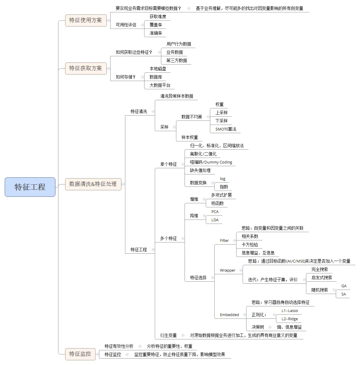
Summary diagram:
My blog will be synced to Tencent Cloud Developer Community—join us: https://cloud.tencent.com/developer/support-plan