Machine Learning (16) — EM Algorithm

Algorithm idea: MLE with hidden variables

We often estimate model parameters from observed samples by maximizing log-likelihood. When data include unobserved latent variables, both latents and parameters are unknown—we cannot maximize log-likelihood directly. EM helps. First, review MLE.

Maximum likelihood estimation (MLE)

Example: hunting with a friend—a rabbit is shot once and falls. Who fired? One shot, one hit—the hunter usually has higher hit rate, so we guess the hunter. That is MLE thinking.

MLE: given outcomes, find parameters that maximize the probability of those outcomes. “Model fixed, parameters unknown.” Steps:

（1）Write likelihood;

（2）Log-likelihood;

（3）Differentiate, set to zero;

（4）Solve.

EM when latents exist: E-step guess latents; M-step maximize log-likelihood over parameters given that guess. Repeat until convergence.

Each iteration: E then M until parameters stabilize.

K-Means algorithm

K-Means recap:

• Choose k centers a₁…a_k

• Assign each x to nearest center

• Update centers to cluster means:

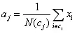
• Repeat until stop (iterations, MSE, center change)

K-Means is intuitive EM: cluster centroids are latents; initialize k centroids (E), assign and update means (M). See K-Means clustering.

Real problems need precise math.

EM algorithm

Example: 50 boys and 50 girls, heights N(μ₁,σ₁) and N(μ₂,σ₂)—MLE per group if labels known. If 100 heights are mixed and unlabeled, we need EM.

Zhihu walkthrough: https://www.zhihu.com/question/27976634/answer/39132183

EM iterates: prior beliefs → fractional counts (E) → update proportions (M) until convergence—like splitting candy between two bags by weight until balanced.

Initialize parameters; repeat until convergence:

• E-step: estimate latent distribution / responsibilities;

• M-step: maximize expected log-likelihood for new parameters.

Setup: samples {x⁽¹⁾,…,x⁽ᵐ⁾}; latent z⁽ⁱ⁾ unknown (like cluster id). Estimate θ for p(x,z). Likelihood has latent z:

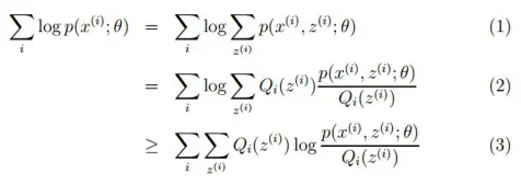
“log of a sum” makes direct differentiation hard. Transform to (2)(3)—Jensen’s inequality:

Convex f: E[f(X)] ≥ f(E[X]); equality for constant X.

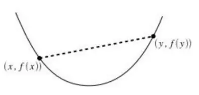
(2) and (3) are inequalities unless we maximize lower bound J until L(θ) is tight.

Fix θ, adjust Q(z) to raise J to L at θ; fix Q, optimize θ (θ_t → θ_{t+1}); repeat to θ*.

Equality in Jensen when

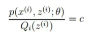
Since

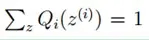
(Q is density over z), numerator sums to c, hence

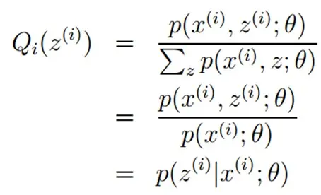
E-step: Q(z) = posterior of latents. M-step: maximize J w.r.t. θ.

EM (Expectation-Maximization): MLE with incomplete data / missing latents.

Algorithm

Initialize θ;

Repeat until convergence:

E-step: posterior / responsibility for latents:

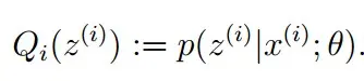
M-step: maximize expected complete log-likelihood:

Iterate until L(θ) is maximized.

Example

Hand-implemented EM for 2-component GMM:

#-*- conding:utf-8 -*-
# --encoding:utf-8 --
"""
Implement GMM clustering via EM
http://scipy.github.io/devdocs/generated/scipy.stats.multivariate_normal.html#scipy.stats.multivariate_normal
"""
import numpy as np
from scipy.stats import multivariate_normal

def train(x, max_iter=100):
    """
    Train 2-component GMM; return (pi, mu1, mu2, sigma1, sigma2)
    :param x: feature matrix
    :param max_iter: max iterations
    :return: (pi, mu1, mu2, sigma1, sigma2)
    """
    m, n = np.shape(x)

    mu1 = x.min(axis=0)
    mu2 = x.max(axis=0)
    sigma1 = np.identity(n)
    sigma2 = np.identity(n)
    pi = 0.5

    for i in range(max_iter):
        norm1 = multivariate_normal(mu1, sigma1)
        norm2 = multivariate_normal(mu2, sigma2)

        # E step
        tau1 = pi * norm1.pdf(x)
        tau2 = (1 - pi) * norm2.pdf(x)
        w = tau1 / (tau1 + tau2)

        # M step
        mu1 = np.dot(w, x) / np.sum(w)
        mu2 = np.dot(1 - w, x) / np.sum(1 - w)
        sigma1 = np.dot(w * (x - mu1).T, (x - mu1)) / np.sum(w)
        sigma2 = np.dot((1 - w) * (x - mu2).T, (x - mu2)) / np.sum(1 - w)
        pi = np.sum(w) / m

    return (pi, mu1, mu2, sigma1, sigma2)

if __name__ == '__main__':
    np.random.seed(28)

    mean1 = (0, 0, 0)
    cov1 = np.diag((1, 1, 1))
    data1 = np.random.multivariate_normal(mean=mean1, cov=cov1, size=500)

    mean2 = (2, 2, 3)
    cov2 = np.array([[1, 1, 3], [1, 2, 1], [0, 0, 1]])
    data2 = np.random.multivariate_normal(mean=mean2, cov=cov2, size=200)

    data = np.vstack((data1, data2))

    pi, mu1, mu2, sigma1, sigma2 = train(data, 100)
    print("第一个类别的相关参数:")
    print(mu1)
    print(sigma1)
    print("第二个类别的相关参数:")
    print(mu2)
    print(sigma2)

    print("预测样本属于那个类别(概率越大就是那个类别)：")
    norm1 = multivariate_normal(mu1, sigma1)
    norm2 = multivariate_normal(mu2, sigma2)
    x = np.array([0, 1, 0])
    print(pi * norm1.pdf(x)) # class 1: ~0.989
    print((1 - pi) * norm2.pdf(x))# class 2: ~0.011

Output:

第一个类别的相关参数:
[-0.03813579 -0.0265211   0.06435217]
[[ 0.89477712 -0.01408823 -0.0630486 ]
 [-0.01408823  1.04926061  0.05625028]
 [-0.0630486   0.05625028  1.01136971]]
第二个类别的相关参数:
[1.89859865 1.9345104  2.77821259]
[[0.84837261 1.11138647 1.12554675]
 [1.11138647 2.19189624 1.37848616]
 [1.12554675 1.37848616 3.43711088]]
预测样本属于那个类别(概率越大就是那个类别)：
0.02758258224417439
0.00039921371592994276

Process finished with exit code 0