Writing

Machine Learning (12) — Random Forest

Ensemble learning, random forest construction, and a cervical cancer risk prediction example.

Preface: With several algorithms covered, this chapter combines them into stronger classifiers via ensemble learning.

Ensemble learning

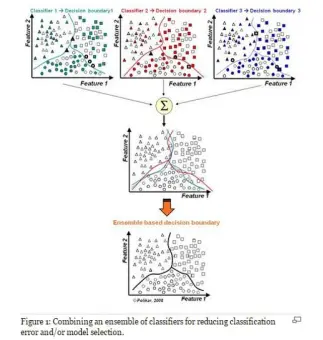
Ensemble learning combines multiple learners (classifiers or regressors) into one. A weak learner beats random guessing only slightly (error rate

Random forest

Random forest modifies Bagging. “Random” means:

（1）Randomness in data (bootstrap samples)

（2）Randomness in features at each split

Diverse trees improve ensemble performance. Data randomness makes trees generalize across scenarios.

Construction workflow

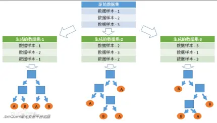
Bootstrap subsamples (with replacement), same size; elements may repeat across/in subsets.

Each subsample trains a tree; each tree votes.

Majority vote is the forest prediction.

Steps:

（1）Bootstrap n samples from training set;

（2）Randomly pick K of all attributes; best split among K;

（3）Repeat m times → m trees;

（4）Majority vote for class.

Note: with-replacement bags often >70% accuracy; without replacement ~60%+.

Example: 3 trees, 2 vote A, 1 votes B → forest predicts A.

Feature randomization

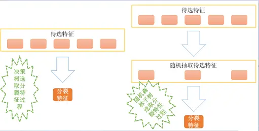
（1）Each tree draws a random feature subset.

（2）Best split among that subset only.

Blue = all candidate features; yellow = chosen split features. Left: single tree uses all features each split. Right: random forest subtree.

Random forest extensions

(Section placeholder in original.)

Algorithm summary

Pros

Parallel training—fast on large data;
Random feature subsets—works with high dimension;
Feature importance;
Bootstrap → lower variance, good generalization;
Simple to implement;
Robust to missing features.

Cons

Can overfit noisy features;
High-cardinality splits dominate—may hurt quality.

Example: breast cancer prediction

ML aids medicine. Example: risk factors → cervical cancer probability.

Collect data from a public dataset:

http://archive.ics.uci.edu/ml/datasets/Cervical+cancer+(Risk+Factors)

Target and features include:

u'Age', u'Number of sexual partners', u'First sexual intercourse',         u'Num of pregnancies', u'Smokes', u'Smokes (years)',         u'Smokes (packs/year)', u'Hormonal Contraceptives',         u'Hormonal Contraceptives (years)', u'IUD', u'IUD (years)', u'STDs',         u'STDs (number)', u'STDs:condylomatosis',         u'STDs:cervical condylomatosis', u'STDs:vaginal condylomatosis',         u'STDs:vulvo-perineal condylomatosis', u'STDs:syphilis',         u'STDs:pelvic inflammatory disease', u'STDs:genital herpes',         u'STDs:molluscum contagiosum', u'STDs:AIDS', u'STDs:HIV',         u'STDs:Hepatitis B', u'STDs:HPV', u'STDs: Number of diagnosis',         u'STDs: Time since first diagnosis', u'STDs: Time since last diagnosis',         u'Dx:Cancer', u'Dx:CIN', u'Dx:HPV', u'Dx', u'Hinselmann', u'Schiller',         u'Citology', u'Biopsy'

Model steps:

Imports

# Data, metrics, RandomForest, plotting (ROC/AUC)

import pandas as pd
import numpy as np
import matplotlib.pyplot as plt
import matplotlib as mpl
from sklearn import tree
from sklearn.ensemble import RandomForestClassifier
from sklearn.model_selection import train_test_split
from sklearn.preprocessing import MinMaxScaler,Imputer,LabelBinarizer

from sklearn import metrics
from sklearn.preprocessing import label_binarize
mpl.rcParams['font.sans-serif'] = [u'SimHei']
mpl.rcParams['axes.unicode_minus'] = False

Load data

names = [u'Age', u'Number of sexual partners', u'First sexual intercourse',
       u'Num of pregnancies', u'Smokes', u'Smokes (years)',
       u'Smokes (packs/year)', u'Hormonal Contraceptives',
       u'Hormonal Contraceptives (years)', u'IUD', u'IUD (years)', u'STDs',
       u'STDs (number)', u'STDs:condylomatosis',
       u'STDs:cervical condylomatosis', u'STDs:vaginal condylomatosis',
       u'STDs:vulvo-perineal condylomatosis', u'STDs:syphilis',
       u'STDs:pelvic inflammatory disease', u'STDs:genital herpes',
       u'STDs:molluscum contagiosum', u'STDs:AIDS', u'STDs:HIV',
       u'STDs:Hepatitis B', u'STDs:HPV', u'STDs: Number of diagnosis',
       u'STDs: Time since first diagnosis', u'STDs: Time since last diagnosis',
       u'Dx:Cancer', u'Dx:CIN', u'Dx:HPV', u'Dx', u'Hinselmann', u'Schiller',
       u'Citology', u'Biopsy']
path="datas/risk_factors_cervical_cancer.csv"
df = pd.read_csv(path)
print(df.shape)

print(df.shape)

(858, 36)

Train/test split

x=df.iloc[:,0:-4]
y=df.iloc[:,-4:]

x=x.replace("?", np.NAN)
imputer=Imputer(missing_values="NaN")
x=imputer.fit_transform(x,y)

x_train,x_test,y_train,y_test = train_test_split(x,y,test_size=0.2,random_state=0)
print("训练样本数量:%d,特征属性数目:%d,目标属性数目:%d"%(x_train.shape[0],x_train.shape[1],y_train.shape[1]))

训练样本数量:686,特征属性数目:32,目标属性数目:4

Train and predict

ss = MinMaxScaler()
x_train = ss.fit_transform(x_train)
x_test = ss.transform(x_test)

rf = RandomForestClassifier(n_estimators=50,criterion="gini",max_depth=1,random_state=10)
rf.fit(x_train,y_train)

score = rf.score(x_test,y_test)

Evaluation

print("准确率：%.2f%%"%(score*100))
forest_y_score = rf.predict_proba(x_test)
forest_fpr1, forest_tpr1, _ = metrics.roc_curve(label_binarize(y_test[names[-4]],classes=(0,1,2)).T[0:-1].T.ravel(), forest_y_score[0].ravel())
forest_fpr2, forest_tpr2, _ = metrics.roc_curve(label_binarize(y_test[names[-3]],classes=(0,1,2)).T[0:-1].T.ravel(), forest_y_score[1].ravel())
forest_fpr3, forest_tpr3, _ = metrics.roc_curve(label_binarize(y_test[names[-2]],classes=(0,1,2)).T[0:-1].T.ravel(), forest_y_score[2].ravel())
forest_fpr4, forest_tpr4, _ = metrics.roc_curve(label_binarize(y_test[names[-1]],classes=(0,1,2)).T[0:-1].T.ravel(), forest_y_score[3].ravel())
auc1 = metrics.auc(forest_fpr1, forest_tpr1)
auc2 = metrics.auc(forest_fpr2, forest_tpr2)
auc3 = metrics.auc(forest_fpr3, forest_tpr3)
auc4 = metrics.auc(forest_fpr4, forest_tpr4)

print ("Hinselmann目标属性AUC值：", auc1)
print ("Schiller目标属性AUC值：", auc2)
print ("Citology目标属性AUC值：", auc3)
print ("Biopsy目标属性AUC值：", auc4)

准确率：89.53%

Hinselmann目标属性AUC值： 0.984586262844781

Schiller目标属性AUC值： 0.9629867495943752

Citology目标属性AUC值： 0.9453082747431043

Biopsy目标属性AUC值： 0.9642712276906437

ROC curves

plt.figure(figsize=(8, 6), facecolor='w')
plt.plot(forest_fpr1,forest_tpr1,c='r',lw=2,label=u'Hinselmann目标属性,AUC=%.3f' % auc1)
plt.plot(forest_fpr2,forest_tpr2,c='b',lw=2,label=u'Schiller目标属性,AUC=%.3f' % auc2)
plt.plot(forest_fpr3,forest_tpr3,c='g',lw=2,label=u'Citology目标属性,AUC=%.3f' % auc3)
plt.plot(forest_fpr4,forest_tpr4,c='y',lw=2,label=u'Biopsy目标属性,AUC=%.3f' % auc4)
plt.plot((0,1),(0,1),c='#a0a0a0',lw=2,ls='--')
plt.xlim(-0.001, 1.001)
plt.ylim(-0.001, 1.001)
plt.xticks(np.arange(0, 1.1, 0.1))
plt.yticks(np.arange(0, 1.1, 0.1))
plt.xlabel('False Positive Rate(FPR)', fontsize=16)
plt.ylabel('True Positive Rate(TPR)', fontsize=16)
plt.grid(b=True, ls=':')
plt.legend(loc='lower right', fancybox=True, framealpha=0.8, fontsize=12)
plt.title(u'随机森林多目标属性分类ROC曲线', fontsize=18)
plt.show()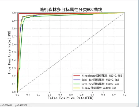

Multiple targets require multi-target evaluation; overall performance is strong.

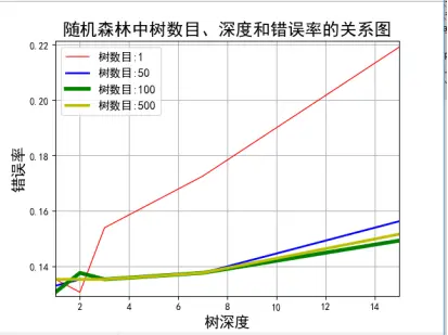
Tree count vs depth

x_train2, x_test2, y_train2, y_test2 = train_test_split(x,y, test_size=0.5, random_state=0)
print("训练样本数量%d，测试样本数量:%d" % (x_train2.shape[0], x_test2.shape[0]))
estimators = [1, 50, 100, 500]
depth = [1, 2, 3, 7, 15]
err_list = []
for es in estimators:
       es_list = []
       for d in depth:
              tf = RandomForestClassifier(n_estimators=es, criterion='gini', max_depth=d, max_features=None,
                                          random_state=0)
              tf.fit(x_train2, y_train2)
              st = tf.score(x_test2, y_test2)
              err = 1 - st
              es_list.append(err)
              print("%d决策树数目，%d最大深度，正确率:%.2f%%" % (es, d, st * 100))
       err_list.append(es_list)

plt.figure(facecolor='w')
i = 0
colors = ['r', 'b', 'g', 'y']
lw = [1, 2, 4, 3]
max_err = 0
min_err = 100
for es, l in zip(estimators, err_list):
       plt.plot(depth, l, c=colors[i], lw=lw[i], label=u'树数目:%d' % es)
       max_err = max((max(l), max_err))
       min_err = min((min(l), min_err))
       i += 1
plt.xlabel(u'树深度', fontsize=16)
plt.ylabel(u'错误率', fontsize=16)
plt.legend(loc='upper left', fancybox=True, framealpha=0.8, fontsize=12)
plt.grid(True)
plt.xlim(min(depth), max(depth))
plt.ylim(min_err * 0.99, max_err * 1.01)
plt.title(u'随机森林中树数目、深度和错误率的关系图', fontsize=18)
plt.show()