Machine Learning (11) — Nonlinear SVM

Preface: The previous chapter on linear SVM left one issue—outliers.

Soft margin

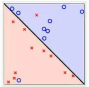
Linear SVM requires linear separability. A few outliers can make the set non-separable even when most data are separable. We add slack η per sample so functional margin can relax, at a cost—misclassification risk. Penalty coefficient C (tuned) limits slack. Smaller C allows more errors (lower train accuracy, often better generalization); larger C forbids errors (higher train accuracy). Outliers in the model:

Then apply formulas from the previous chapter (derivation omitted here).

Soft margin summary

（1）Handles outliers in nearly linear data;

（2）Penalty improves robustness;

（3）Smaller C → more tolerated errors, lower accuracy; larger C → stricter, higher train accuracy.

Both hard-margin and soft-margin linear SVM still need some linear separability (possibly after slack). Fully non-linear data need another approach:

Polynomial expansion

In linear regression, polynomial features map low-D to high-D for linear models. Similarly, 2D non-separable data may become separable in higher dimensions.

2D linear model:

A line:

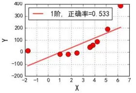
Polynomial expansion:

2D → 5D:

In plots:

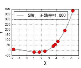
Polynomial expansion maps non-linearly separable data so a hyperplane can split them.

Mapping function

Like polynomial regression for SVM: map to high-D, then use linear or soft-margin SVM. Key: the map from low to high dimension.

How choose the map?

Two concentric rings in 2D: add radius as third coordinate → 3D, separable:

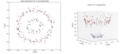
Many maps work—any that linearizes the data.

Define Φ: low-D → high-D. Nonlinear SVM objective (from earlier):

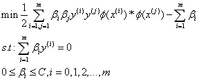
Only dot products need to become dot products in feature space.

Problem solved? Map everything to high-D and run linear SVM? Not quite: 2D → 5D; 3D → 9D; n-D → n(n+3)/2—combinatorial blowup; infinite-D is intractable.

Kernel trick below.

Kernel functions

Kernels compute in low-D what corresponds to high-D dot products—avoid explicit Φ.

If Φ maps low to high and

then K(x,z) is a kernel.

Common kernels: linear, polynomial, Gaussian (RBF), sigmoid—polynomial and RBF most used.

Polynomial kernel:

γ, r, d are hyperparameters.

Example vectors a, b:

5D map:

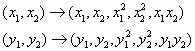
Dot product in 5D:

Similar form in 2D:

Scale to match—polynomial kernel coefficients.

Gaussian (RBF):

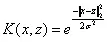
One parameter, covers many mappings—RBF is common in practice.

RBF separation:

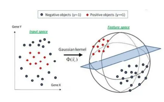
Proof that Gaussian = inner product of maps: https://blog.csdn.net/u010551462/article/details/41748807

Kernel summary

（1）Custom kernels allowed; must be positive definite (Gram matrix PSD);

（2）Low-D computation, linear separability in implicit high-D;

（3）Turns non-linear problems into linearly separable ones in feature space.