Machine Learning (10) — Linear SVM

Support Vector Machine (SVM) is originally a binary classification algorithm—an extension of the perceptron. Modern SVM supports linear and nonlinear classification and can be applied to regression; via OvR or OvO it also handles multiclass problems. Setting aside ensemble methods and dataset specifics, SVM is among the strongest classifiers.

Algorithm Idea

In the perceptron model, the algorithm finds a separating hyperplane so as many points as possible lie on either side for classification—but in real data many such hyperplanes may exist. As shown:

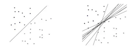
The perceptron can find multiple separating hyperplanes and, when optimizing, wants all points as far from the plane as possible—but points already far enough are usually classified correctly, so pushing them farther is meaningless. What matters are points near the hyperplane, which are easily misclassified. SVM makes those near points stay as far from the hyperplane as possible.

For a simple introduction to SVM concepts, see this Zhihu answer by 简之—vivid analogies for each idea; I won’t repeat them here. Link: https://www.zhihu.com/question/21094489. Linearly separable: if a hyperplane can separate two classes, the dataset is linearly separable. Linearly inseparable: no such hyperplane exists. Separating hyperplane: the line/plane that splits the dataset. Margin: distance from a data point to the separating hyperplane. Support vector: points closest to the separating hyperplane. In the figure below, red and blue marked points are support vectors.

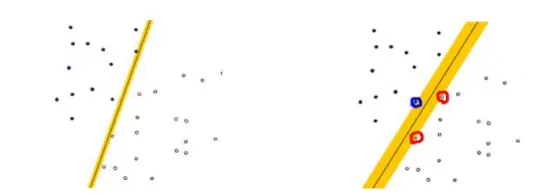
Linearly Separable SVM

SVM finds points closest to the hyperplane and solves for the optimum under constraints. As shown:

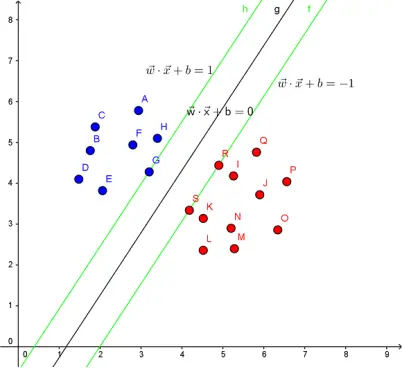
Support vectors satisfy:

Distance from a support vector to the hyperplane:

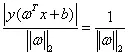
Our approach: keep classified points on either side of support vectors while maximizing margin. The optimization can be written:

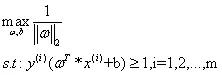
This can be transformed into:

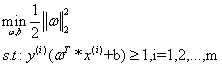
Equivalently, minimize loss J(w):

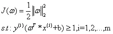
The problem can be solved with KKT conditions as discussed earlier:

Solution process:

After introducing Lagrange multipliers, the objective becomes:

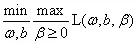
By Lagrangian duality, we convert to an equivalent dual problem:

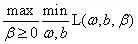
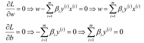
For this objective, first minimize over w and b, then maximize over multipliers. Minimization: set partial derivatives to zero to get parameters.

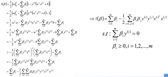
Substituting into L(W, b, β) yields L(β) depending only on β:

Solution process:

After minimizing over W and b, the objective depends only on β; maximize it to get β, then w and b.

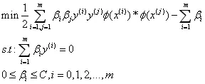
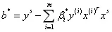
β can be solved with SMO (covered later). Given optimal β*, compute W and b from their relations; b is often the mean over all support vectors. The solution is:

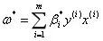
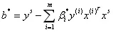
This yields the final SVM classifier.

SVM Algorithm Flow

Input: m linearly separable samples {(x₁,y₁), (x₂,y₂), …, (x_m,y_m)} where x is n-dimensional and y is binary (+1 or −1). Output: parameters w, b, and decision function. Steps:

(1) Formulate the constrained optimization problem;

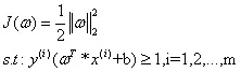
(2) Use SMO to obtain optimal β*; (3) identify support vector set S; (4) update W and b;

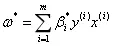
(5) Build the final classifier:

Summary

(1) Data must be linearly separable; (2) purely linearly separable SVM may predict poorly on outliers; (3) for linearly separable data, SVM classification works very well.