Writing
Deep Learning — RBF
RBF is less common, but its local approximation idea enables faster parameter fitting and has promising future directions.
Preface: RBF is not used much, but its idea of local approximation can solve parameters faster and should have a good future.
Introduction
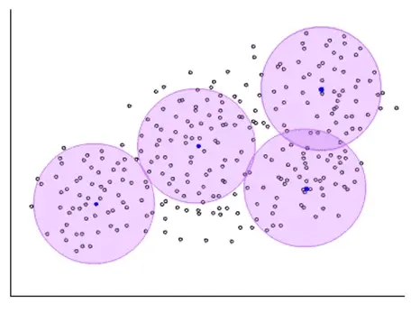
1> Method: Similar to clustering, a few centers are given first; then data is assigned to a center, and features of that center dominate. An RBF network can approximate any nonlinear function, handle hard-to-parse regularities in a system, generalize well, and learn quickly.
2> Advantages: Fast convergence; applied to nonlinear function approximation, time series analysis, classification, pattern recognition, information processing, image processing, system modeling, control, and fault diagnosis.
3> Global approximation network: When one or more tunable parameters (weights or thresholds) affect every output, the network is global—each weight adjusts on every input, so learning is slow (e.g. BP).
4> Local approximation network: When only a few connection weights in a local region of input space affect the output, the network is local (e.g. RBF).
Principle
RBF networks usually have three layers:
1> Input layer
2> Hidden layer: Computes radial basis function (RBF) values from Euclidean distance between input vector x and center vectors c. The hidden layer maps from low-dimensional m to high-dimensional P so that linearly inseparable low-dimensional cases become linearly separable in high dimensions.
3> Output layer: Computes their linear combination.
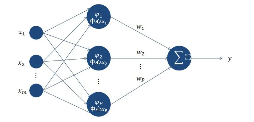
Properties of the RBF kernel:

First, clustering-like steps distinguish memory samples (centers in the figure); then BP-like algorithms solve for parameters.
Problems in neural networks: In general, adding neurons and depth improves learning and fit to data, but depth is often limited in practice because very deep networks can cause optimization issues. In DNN training, two problems may appear: vanishing and exploding gradients. Gradients use the chain rule—a product of terms. If each layer factor is < 1, the product shrinks (vanishing); if each is > 1, it grows (exploding). Code for an RBF network:
from scipy.linalg import norm, pinv
import numpy as np

from matplotlib import pyplot as plt

np.random.seed(28)

class RBF:
    """
    RBF径向基神经网络
    """

    def __init__(self, input_dim, num_centers, out_dim):
        """
        初始化函数
        :param input_dim: 输入维度数目
        :param num_centers: 中间的核数目
        :param out_dim:输出维度数目
        """
        self.input_dim = input_dim
        self.out_dim = out_dim
        self.num_centers = num_centers
        self.centers = [np.random.uniform(-1, 1, input_dim) for i in range(num_centers)]
        self.beta = 8
        self.W = np.random.random((self.num_centers, self.out_dim))

    def _basisfunc(self, c, d):
        return np.exp(-self.beta * norm(c - d) ** 2)

    def _calcAct(self, X):
        # calculate activations of RBFs
        G = np.zeros((X.shape[0], self.num_centers), float)
        for ci, c in enumerate(self.centers):
            for xi, x in enumerate(X):
                G[xi, ci] = self._basisfunc(c, x)
        return G

    def train(self, X, Y):
        """
        进行模型训练
        :param X: 矩阵,x的维度必须是给定的n * input_dim
        :param Y: 列的向量组合,要求维度必须是n * 1
        :return:
        """

        # 随机初始化中心点(permutation API的作用是打乱顺序,如果给定的是一个int类型的数据,那么打乱range(int)序列)
        rnd_idx = np.random.permutation(X.shape[0])[:self.num_centers]
        self.centers = [X[i, :] for i in rnd_idx]

        # calculate activations of RBFs
        # 相当于计算RBF中的激活函数值
        G = self._calcAct(X)

        # calculate output weights (pseudoinverse)
        # 计算权重(pinv API:计算矩阵的逆) ==> Y=GW ==> W = G^-1Y
        self.W = np.dot(pinv(G), Y)

    def test(self, X):
        """ X: matrix of dimensions n x indim """
        G = self._calcAct(X)
        Y = np.dot(G, self.W)
        return Y

# 构造数据
n = 100
x = np.linspace(-1, 1, n).reshape(n, 1)
y = np.sin(3 * (x + 0.5) ** 3 - 1)
# y = y + np.random.normal(0, 0.1, n).reshape(n, 1)

# RBF神经网络
rbf = RBF(1, 10, 1)
rbf.train(x, y)
z = rbf.test(x)

# plot original data
plt.figure(figsize=(12, 8))
# 展示原始值,黑色
plt.plot(x, y, 'k-')

# plot learned model
# 展示预测值
plt.plot(x, z, 'r-', linewidth=2)

plt.xlim(-1.2, 1.2)
plt.show()
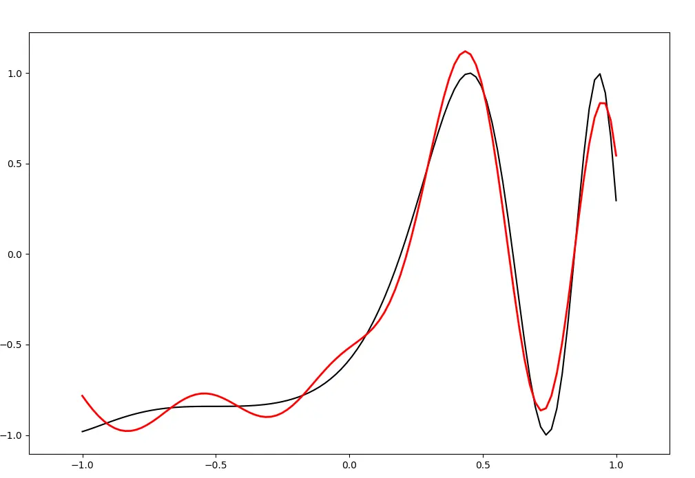
Result: