Deep Learning — Backpropagation

Preface: Starting from the perceptron, we introduce neurons, improve the activation function in the perceptron, introduce fully connected neural networks, and focus on backpropagation (BP) neural networks.

Perceptron Neural Network

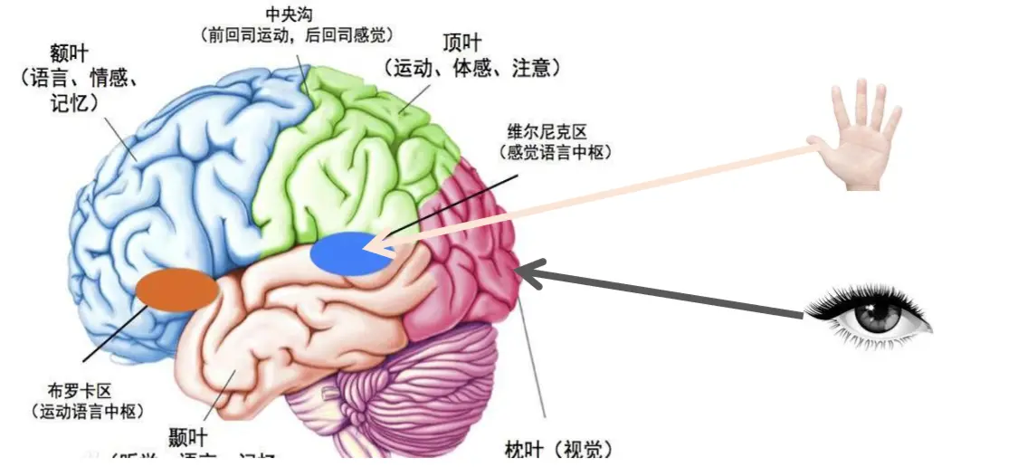
Also called a 0/1 classifier: given a threshold, it solves binary classification. Similar to binarization mentioned earlier—for example, when ranking scores, scores above 60 are labeled “pass.” Adding “excellent” for scores above 80 only requires another perceptron. Since neural networks simulate human thinking—given an input, they produce an output—human decisions are the result of many neurons. Below we analyze what a simple perceptron network produces for classification. The brain is distributed as shown below:

• Neuron As mentioned before, briefly: input, output, and activation function. 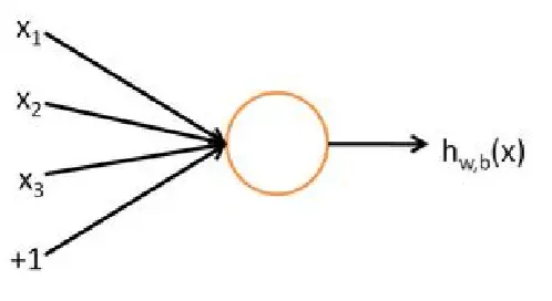Perceptron When the activation function returns only two values, it is a perceptron. Drawback: Because the output is fixed to two values, during parameter optimization the output either stays unchanged or jumps suddenly, making optimization difficult. Sigmoid is usually used as the activation function instead.

Linear Neural Network

Can handle multi-class problems. A neural network with a small number of hidden layers is called a shallow neural network, also known as a traditional neural network—typically one with two hidden layers. The downside of sigmoid is that hidden layers are effectively limited to two: because of the special properties of the activation function, during iterative differentiation the sigmoid derivative tends toward zero, causing “dead neurons.”

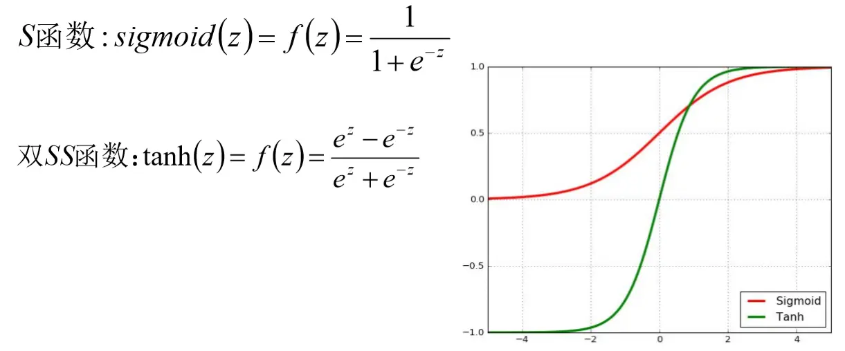
Note the range and trend of the function in the figure. tanh works somewhat better but still cannot solve the problem of many hidden layers, so ReLU was introduced later.

BP Neural Network

An algorithm for solving W in neural networks, split into forward propagation (FP) to compute loss and backpropagation (BP) to pass errors backward; weights at each layer are updated from the error, then iteration continues. Traditional neural networks are not used much: with too few layers they underperform SVM; with too many layers they are hard to train. Convolutional neural networks were introduced later. Below is a diagram of forward propagation for loss and backpropagation for error, used to update parameters w:

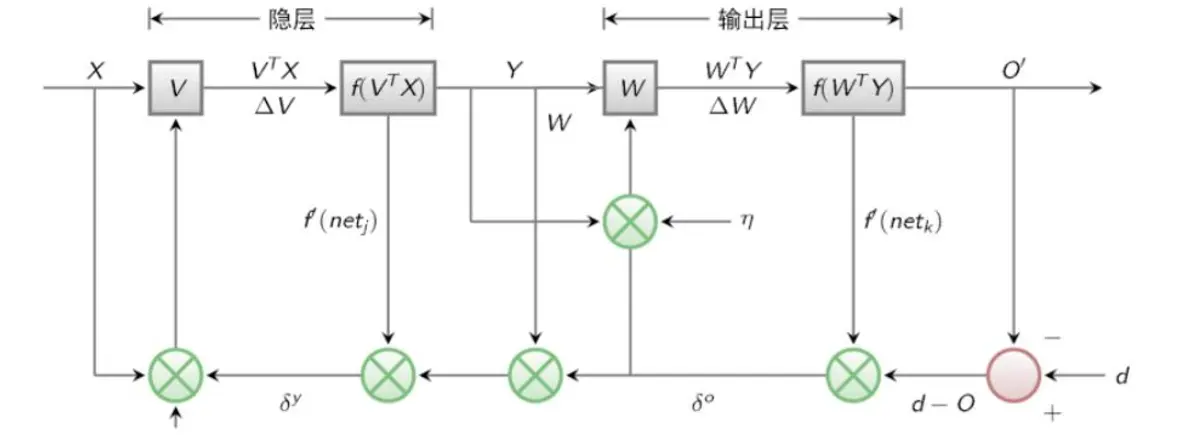
Note: net refers to the linear transform of inputs; f(net) applies the activation function; d is the label; O is the network prediction. Output layer error:

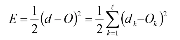
Hidden layer error:

Input layer error:

Code implementing the BP algorithm:

import numpy as np

w = [0.1, 0.15, 0.2, 0.25, 0.3, 0.35, 0.4, 0.45, 0.5, 0.55, 0.6, 0.65]
# 偏置项b不进行更新
b = [0.35, 0.65]
l = [-5, 10]

def sigmoid(z):
    return 1.0 / (1 + np.exp(-z))

def f1(w, b, l):
    # 前向传播，计算结果值
    h1 = sigmoid(w[0] * l[0] + w[1] * l[1] + b[0])
    h2 = sigmoid(w[2] * l[0] + w[3] * l[1] + b[0])
    h3 = sigmoid(w[4] * l[0] + w[5] * l[1] + b[0])

    o1 = sigmoid(w[6] * h1 + w[8] * h2 + w[10] * h3 + b[1])
    o2 = sigmoid(w[7] * h1 + w[9] * h2 + w[11] * h3 + b[1])

    # 后向传播，更新w
    t1 = -(0.1 - o1) * o1 * (1 - o1)
    t2 = -(0.99 - o2) * o2 * (1 - o2)

    w[6] = w[6] - 0.5 * (t1 * h1)
    w[8] = w[8] - 0.5 * (t1 * h2)
    w[10] = w[10] - 0.5 * (t1 * h3)
    w[7] = w[7] - 0.5 * (t2 * h1)
    w[9] = w[9] - 0.5 * (t2 * h2)
    w[11] = w[11] - 0.5 * (t2 * h3)

    w[0] = w[0] - 0.5 * (t1 * w[6] + t2 * w[7]) * h1 * (1 - h1) * l[0]
    w[1] = w[1] - 0.5 * (t1 * w[6] + t2 * w[7]) * h1 * (1 - h1) * l[1]
    w[2] = w[2] - 0.5 * (t1 * w[8] + t2 * w[9]) * h2 * (1 - h2) * l[0]
    w[3] = w[3] - 0.5 * (t1 * w[8] + t2 * w[9]) * h2 * (1 - h2) * l[1]
    w[4] = w[4] - 0.5 * (t1 * w[10] + t2 * w[11]) * h3 * (1 - h3) * l[0]
    w[5] = w[5] - 0.5 * (t1 * w[10] + t2 * w[11]) * h3 * (1 - h3) * l[1]

    return o1, o2, w

for i in range(1001):
    r1, r2, w = f1(w, b, l)
    print("第{}次迭代后，结果值为:({},{}),权重更新为:{}".format(i, r1, r2, w))

Output:

第1000次迭代后，结果值为:(0.09996083954832574,0.9778184034399262),权重更新为:[-0.030672263069416547, 0.41134452613883266, 0.09476393030400698, 0.4604721393919862, 0.20319883709854172, 0.5436023258029161, -0.9980730809431909, 0.9438220932399313, -0.8629482660589612, 1.0419668423034139, -1.0146000749780355, 1.181504874794456]